Code
library(mlr3verse)mlr3: Basics{mlr3} is structured (Lang et al. 2019)learners and (built-in) tasksTo get started, we load {mlr3verse}, which will load various packages from the {mlr3} ecosystem:
library(mlr3verse){mlr3} ships with wrappers for many commonly used machine learning algorithms (“learners”).
We can access the list of available learners using the mlr_learners dictionary:
sample(mlr_learners$keys(), 10) [1] "classif.decision_table" "classif.abess" "surv.bart"
[4] "clust.diana" "classif.ctree" "classif.catboost"
[7] "classif.random_tree" "dens.nonpar" "classif.earth"
[10] "surv.mboost" One example:
lrn("classif.ranger")<LearnerClassifRanger:classif.ranger>: Random Forest
* Model: -
* Parameters: num.threads=1
* Packages: mlr3, mlr3learners, ranger
* Predict Types: [response], prob
* Feature Types: logical, integer, numeric, character, factor, ordered
* Properties: hotstart_backward, importance, multiclass, oob_error,
twoclass, weightsUse lrn("classif.ranger")$help() to view the help page, with links to documentation for parameters and other information about the wrapped learner.
Built-in tasks can be accessed using the mlr_tasks dictionary:
head(as.data.table(mlr_tasks)[, list(key, label, task_type, nrow, ncol, properties)])Key: <key>
key label task_type nrow ncol properties
<char> <char> <char> <int> <int> <list>
1: ames_housing Ames House Sales regr 2930 82
2: bike_sharing Bike Sharing Demand regr 17379 14
3: boston_housing Boston Housing Prices regr 506 18
4: breast_cancer Wisconsin Breast Cancer classif 683 10 twoclass
5: german_credit German Credit classif 1000 21 twoclass
6: ilpd Indian Liver Patient Data classif 583 11 twoclassOne example:
tsk("penguins_simple")<TaskClassif:penguins> (333 x 11): Simplified Palmer Penguins
* Target: species
* Properties: multiclass
* Features (10):
- dbl (7): bill_depth, bill_length, island.Biscoe, island.Dream,
island.Torgersen, sex.female, sex.male
- int (3): body_mass, flipper_length, yearTasks encapsulate a data source (typically a data.table) and additional information regarding which variables are considered features and target. Tasks can also specify additional properties such as stratification, which we will see later.
task and learnerThe below code snippet trains a random forest model on the penguins_simple task (a simplified version of the palmerpenguins dataset, but without missing values) and evaluates the model’s performance using the classification error metric:
task = tsk("penguins_simple")
learner = lrn("classif.ranger", num.trees = 10)

part = partition(task, ratio = 0.8) # by default stratifies on the target column

learner$train(task, row_ids = part$train)
preds = learner$predict(task, row_ids = part$test)
preds$score(msr("classif.ce"))
classif.ce
0.01492537 Learn more by reading the respective chapter on the mlr3 book.
mlr3proba: Basics{mlr3proba} (Sonabend et al. 2021){mlr3proba} extends {mlr3} with survival analysis capabilities.
As of now, {mlr3proba} is not on CRAN, but you can install it from GitHub or r-universe. More info is also available on the respective mlr3 book chapter.
We’ll start by using the built-in lung dataset, which is a survival task with 7 features and 168 observations:
library(mlr3proba)
task = tsk("lung")

task
<TaskSurv:lung> (168 x 9): Lung Cancer
* Target: time, status
* Properties: -
* Features (7):
- int (6): age, meal.cal, pat.karno, ph.ecog, ph.karno, wt.loss
- fct (1): sexSee online reference to useful methods offered by the main TaskSurv class. Some examples:
Target Surv object from {survival} (+ denotes censored observation):
head(task$truth())[1] 455 210 1022+ 310 361 218 Proportion of censored observations:
task$cens_prop()[1] 0.2797619Does the data satisfy the proportional hazards assumption? Get the p-value from the Grambsch-Therneau test (see ?survival::cox.zph (Grambsch and Therneau 1994)):
task$prop_haz() # barely, p > 0.05 => PH[1] 0.0608371Using the autoplot() function from {ggplot2}, we get the Kaplan-Meier curve:
library(ggplot2)
autoplot(task) +
labs(title = "Lung dataset: Kaplan-Meier curve")Registered S3 method overwritten by 'GGally':
method from
+.gg ggplot2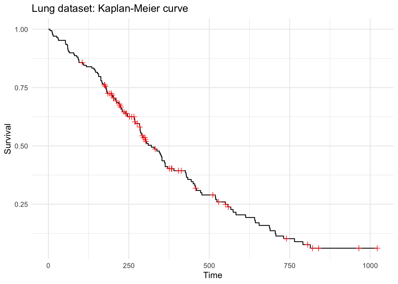
Tasks shipped with {mlr3proba}:
as.data.table(mlr_tasks)[task_type == "surv", list(key, label, nrow, ncol)]Key: <key>
key label nrow ncol
<char> <char> <int> <int>
1: actg ACTG 320 1151 13
2: gbcs German Breast Cancer 686 10
3: gbsg German Breast Cancer 686 10
4: grace GRACE 1000 1000 8
5: lung Lung Cancer 168 9
6: mgus MGUS 176 9
7: pbc Primary Biliary Cholangitis 276 19
8: rats Rats 300 5
9: unemployment Unemployment Duration 3343 6
10: veteran Veteran 137 8
11: whas Worcester Heart Attack 481 11TaskSurv objecttsk("lung")$help() to get more info about the dataset and pre-processing appliedThe classical Cox Proportional Hazards model:
cox = lrn("surv.coxph")
cox<LearnerSurvCoxPH:surv.coxph>: Cox Proportional Hazards
* Model: -
* Parameters: list()
* Packages: mlr3, mlr3proba, survival, distr6
* Predict Types: [crank], distr, lp
* Feature Types: logical, integer, numeric, factor
* Properties: weightsTrain the cox model and access the fit object from the {survival} package:
set.seed(42)
part = partition(task, ratio = 0.8) # by default, stratification is on `status` variable
cox$train(task, row_ids = part$train)
cox$modelCall:
survival::coxph(formula = task$formula(), data = task$data(),
x = TRUE)
coef exp(coef) se(coef) z p
age 1.341e-02 1.013e+00 1.258e-02 1.066 0.2864
meal.cal -5.007e-05 9.999e-01 2.903e-04 -0.172 0.8631
pat.karno -2.142e-02 9.788e-01 9.055e-03 -2.366 0.0180
ph.ecog 5.936e-01 1.811e+00 2.500e-01 2.375 0.0176
ph.karno 2.541e-02 1.026e+00 1.263e-02 2.011 0.0443
sexm 4.510e-01 1.570e+00 2.298e-01 1.962 0.0497
wt.loss -1.500e-02 9.851e-01 8.395e-03 -1.787 0.0739
Likelihood ratio test=23.36 on 7 df, p=0.001475
n= 135, number of events= 97 Visual output of the model, using the latest version from Github of {mlr3viz}:
autoplot(cox)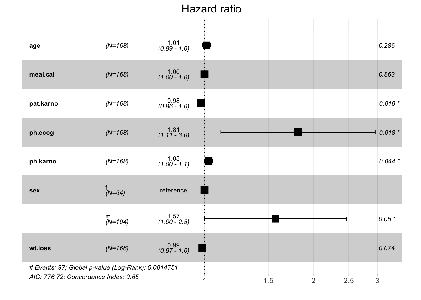
Let’s predict using the trained cox model on the test set (output is a PredictionSurv object):
p = cox$predict(task, row_ids = part$test)
p<PredictionSurv> for 33 observations:
row_ids time status crank lp distr
1 455 TRUE -0.16022736 -0.16022736 <list[1]>
8 170 TRUE 0.07608537 0.07608537 <list[1]>
15 371 TRUE -0.46601841 -0.46601841 <list[1]>
---
165 191 FALSE -0.30526841 -0.30526841 <list[1]>
166 105 FALSE 0.49632782 0.49632782 <list[1]>
168 177 FALSE -0.17234336 -0.17234336 <list[1]>crank: Continuous risk rankinglp: Linear predictor calculated as \hat\beta * X_{test}distr: Predicted survival distribution, either discrete or continuousresponse: Predicted survival timeFor the cox model, crank = lp (the higher, the more risk):
p$lp 1 2 3 4 5 6
-0.160227364 0.076085366 -0.466018411 0.293380270 1.179147761 0.523244848
7 8 9 10 11 12
0.391564618 -0.029833700 -0.149489235 -0.262762070 0.076021387 0.279388934
13 14 15 16 17 18
0.889995280 0.859467193 1.030472975 0.277533930 -0.057165655 0.362416853
19 20 21 22 23 24
-0.037670338 -0.295071061 -0.419840184 0.793214751 0.823500785 0.977222024
25 26 27 28 29 30
-0.046252611 0.021227170 -0.093541236 -0.158438686 1.615114453 0.003701068
31 32 33
-0.305268413 0.496327822 -0.172343361 Survival prediction is a 2D matrix essentially, with dimensions: observations x time points:
p$data$distr[1:5, 1:5] 5 11 12 13 15
1 0.9959775 0.9919519 0.9879072 0.9837970 0.9796477
2 0.9949079 0.9898175 0.9847084 0.9795222 0.9742926
3 0.9970357 0.9940659 0.9910789 0.9880402 0.9849691
4 0.9936759 0.9873617 0.9810323 0.9746156 0.9681535
5 0.9847342 0.9696296 0.9546262 0.9395560 0.9245212Users should use the distr6 interface (Sonabend and Kirdly 2021) to access this prediction type, which allows us to retrieve survival probabilities (or hazards) for any time point of interest:
# first 4 patients in the test set, specific time points:
p$distr[1:4]$survival(c(100, 500, 1200)) [,1] [,2] [,3] [,4]
100 0.9184997 0.8979186 0.9393041 0.87475634
500 0.4589611 0.3729197 0.5634874 0.29352281
1200 0.1684876 0.1048078 0.2693617 0.06062239Visualization of predicted survival curves for 3 test patients:
p2 = p$clone()$filter(row_ids = c(1,24,40))
autoplot(p2, type = "preds")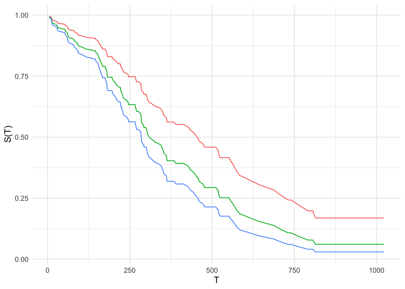
Validation of a survival model can be done by assessing:
Many measures included in mlr3proba:
mlr_measures$keys(pattern = "surv") [1] "surv.brier" "surv.calib_alpha" "surv.calib_beta"
[4] "surv.chambless_auc" "surv.cindex" "surv.dcalib"
[7] "surv.graf" "surv.hung_auc" "surv.intlogloss"
[10] "surv.logloss" "surv.mae" "surv.mse"
[13] "surv.nagelk_r2" "surv.oquigley_r2" "surv.rcll"
[16] "surv.rmse" "surv.schmid" "surv.song_auc"
[19] "surv.song_tnr" "surv.song_tpr" "surv.uno_auc"
[22] "surv.uno_tnr" "surv.uno_tpr" "surv.xu_r2" Most commonly used metrics are for assessing discrimination, such as Harrell’s C-index (Harrell et al. 1982), Uno’s C-index (Uno et al. 2011) and the (time-dependent) AUC (Heagerty and Zheng 2005; Uno et al. 2007):
harrell_c = msr("surv.cindex", id = "surv.cindex.harrell")
uno_c = msr("surv.cindex", weight_meth = "G2", id = "surv.cindex.uno")
uno_auci = msr("surv.uno_auc", integrated = TRUE) # across all times in the test set
uno_auc = msr("surv.uno_auc", integrated = FALSE, times = 10) # at a specific time-point of interest
harrell_c<MeasureSurvCindex:surv.cindex.harrell>
* Packages: mlr3, mlr3proba
* Range: [0, 1]
* Minimize: FALSE
* Average: macro
* Parameters: weight_meth=I, tiex=0.5, eps=0.001
* Properties: -
* Predict type: crank
* Return type: Scoreuno_auc<MeasureSurvUnoAUC:surv.uno_auc>
* Packages: mlr3, mlr3proba, survAUC
* Range: [0, 1]
* Minimize: FALSE
* Average: macro
* Parameters: integrated=FALSE, times=10
* Properties: requires_task, requires_train_set
* Predict type: lp
* Return type: Scorecrank or lp predictionp$score(harrell_c)surv.cindex.harrell
0.6336898 p$score(uno_c, task = task, train_set = part$train)surv.cindex.uno
0.5907828 Calibration is traditionally performed graphically via calibration plots:
autoplot(p, type = "calib", task = task, row_ids = part$test)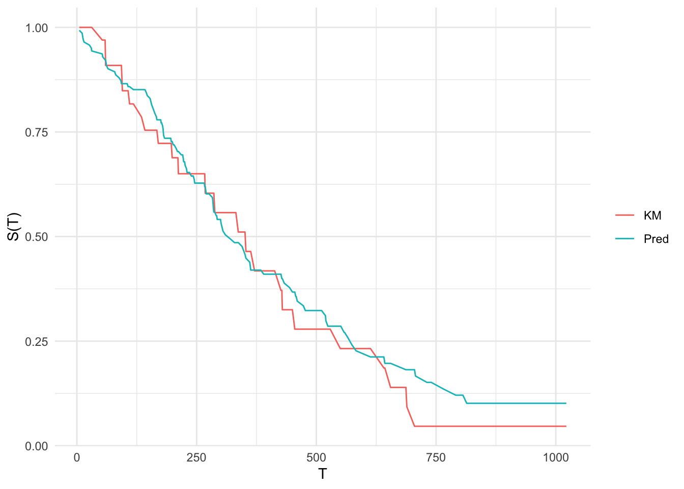
But there exists also calibration metrics, e.g. D-Calibration (Haider et al. 2020):
dcal = msr("surv.dcalib")
dcal<MeasureSurvDCalibration:surv.dcalib>
* Packages: mlr3, mlr3proba
* Range: [0, Inf]
* Minimize: TRUE
* Average: macro
* Parameters: B=10, chisq=FALSE, truncate=Inf
* Properties: -
* Predict type: distr
* Return type: Scorep$score(dcal)surv.dcalib
8.320423 Overall survival prediction performance can be assessed by scoring rules such as the Integrated Survival Brier Score (ISBS) (Graf et al. 1999) and the Right-censored Log-Loss (RCLL) (Avati et al. 2020) among others:
rcll = msr("surv.rcll")
rcll<MeasureSurvRCLL:surv.rcll>
* Packages: mlr3, mlr3proba, distr6
* Range: [0, Inf]
* Minimize: TRUE
* Average: macro
* Parameters: eps=1e-15, se=FALSE, ERV=FALSE, na.rm=TRUE
* Properties: -
* Predict type: distr
* Return type: Scorep$score(rcll)surv.rcll
23.46684 ibrier = msr("surv.brier", proper = TRUE)
ibrier<MeasureSurvGraf:surv.graf>
* Packages: mlr3, mlr3proba
* Range: [0, Inf]
* Minimize: TRUE
* Average: macro
* Parameters: integrated=TRUE, method=2, se=FALSE, proper=TRUE,
eps=0.001, ERV=FALSE
* Properties: -
* Predict type: distr
* Return type: Scorep$score(ibrier, task = task, train_set = part$train)surv.graf
0.1591112 resample()auto_tuner()So far we have used the Cox regression model, but there are many more machine learning methods available via mlr3extralearners (learner list)! We will take a look at the following:
glmnet (Friedman, Hastie, and Tibshirani 2010)
lrn("surv.cv_glmnet"), wich internally tunes for lambda using cross-validationCoxBoost (Binder and Schumacher 2008)
lrn("surv.cv_coxboost", penalty = "optimCoxBoostPenalty"), which also uses internal cross-validation to tune its parametersranger (Ishwaran et al. 2008)aorsf (Jaeger et al. 2023)These learners then cover the range from penalized regression to tree ensembles and boosting.
Let’s take these learners for a spin on a subset of TCGA breast cancer data with gene expression and clinical features. We first need to create a TaskSurv object from the data, which we can do by reading in the data and then using as_task_surv(). We also add the status column to the stratum, which is necessary for the resampling to ensure a similar proportion of events in the resampling folds with the complete dataset.
tcga = readRDS("data/tcga.rds")
task_tcga = mlr3proba::as_task_surv(
x = tcga,
time = "time", event = "status", id = "BRCA-TCGA"
)
# Set stratum for resampling
task_tcga$set_col_roles("status", add_to = "stratum")
task_tcga<TaskSurv:BRCA-TCGA> (1047 x 54)
* Target: time, status
* Properties: strata
* Features (52):
- dbl (52): ACTR3B, ANLN, BAG1, BCL2, BIRC5, BLVRA, CCNB1, CCNE1,
CDC20, CDC6, CDH3, CENPF, CEP55, CXXC5, EGFR, ERBB2, ESR1, EXO1,
FGFR4, FOXA1, FOXC1, GPR160, GRB7, KIF2C, KRT14, KRT17, KRT5, MAPT,
MDM2, MELK, MIA, MKI67, MLPH, MMP11, MYBL2, MYC, NAT1, NDC80, NUF2,
ORC6, PGR, PHGDH, PTTG1, RRM2, SFRP1, SLC39A6, TMEM45B, TYMS,
UBE2C, UBE2T, age, ethnicity
* Strata: statusWe can instantiate our learners as we’ve seen before — we’re sticking to mostly vanilla settings for now.
We can let glmnet determine the optimal value for lambda with it’s internal cross-validation method Similarly, CoxBoost could tune itself, but we’ll stick with a simple version to save some time on compute! For the forests, we use 100 trees each for speed and otherwise accept the defaults.
To speed things up a little, we let learners use 4 parallel threads (num.threads in ranger and n_thread in aorsf), which you may want to change depending on your available resources!
lrn_glmnet = lrn("surv.cv_glmnet", alpha = 0.5, s = "lambda.min")
lrn_coxboost = lrn("surv.coxboost", penalty = 100)
lrn_ranger = lrn("surv.ranger", num.trees = 100, num.threads = 4)
lrn_aorsf = lrn("surv.aorsf", n_tree = 100, n_thread = 4)We can now use resample() to evaluate the performance of each of these learners on the task. To do this, we decide on two measures: Harrell’s C and the integrated brier score, and we also instantiate a resampling to use for comparison, such that we ensure all learners see the same data.
measures = list(msr("surv.cindex", id = "cindex"), msr("surv.brier", id = "ibs"))
resampling = rsmp("cv", folds = 3)
resampling$instantiate(task_tcga)
rr_glmnet = resample(
task = task_tcga,
learner = lrn_glmnet,
resampling = resampling
)INFO [00:10:58.085] [mlr3] Applying learner 'surv.cv_glmnet' on task 'BRCA-TCGA' (iter 1/3)
INFO [00:10:59.532] [mlr3] Applying learner 'surv.cv_glmnet' on task 'BRCA-TCGA' (iter 2/3)
INFO [00:11:00.649] [mlr3] Applying learner 'surv.cv_glmnet' on task 'BRCA-TCGA' (iter 3/3)rr_glmnet$score(measures) task_id learner_id resampling_id iteration cindex ibs
<char> <char> <char> <int> <num> <num>
1: BRCA-TCGA surv.cv_glmnet cv 1 0.5336199 0.1428582
2: BRCA-TCGA surv.cv_glmnet cv 2 0.7011343 0.2703538
3: BRCA-TCGA surv.cv_glmnet cv 3 0.7201999 0.1859438
Hidden columns: task, learner, resampling, predictionFeel free to play with the parameters of glmnet a bit more — for example, does changing alpha help?
We can repeat the same procedure for the other learners:
rr_coxboost = resample(
task = task_tcga,
learner = lrn_coxboost,
resampling = resampling
)INFO [00:11:02.267] [mlr3] Applying learner 'surv.coxboost' on task 'BRCA-TCGA' (iter 1/3)
INFO [00:11:02.915] [mlr3] Applying learner 'surv.coxboost' on task 'BRCA-TCGA' (iter 2/3)
INFO [00:11:03.630] [mlr3] Applying learner 'surv.coxboost' on task 'BRCA-TCGA' (iter 3/3)rr_ranger = resample(
task = task_tcga,
learner = lrn_ranger,
resampling = resampling
)INFO [00:11:04.357] [mlr3] Applying learner 'surv.ranger' on task 'BRCA-TCGA' (iter 1/3)
INFO [00:11:05.167] [mlr3] Applying learner 'surv.ranger' on task 'BRCA-TCGA' (iter 2/3)
INFO [00:11:05.962] [mlr3] Applying learner 'surv.ranger' on task 'BRCA-TCGA' (iter 3/3)rr_aorsf = resample(
task = task_tcga,
learner = lrn_aorsf,
resampling = resampling
)INFO [00:11:06.876] [mlr3] Applying learner 'surv.aorsf' on task 'BRCA-TCGA' (iter 1/3)
INFO [00:11:07.004] [mlr3] Applying learner 'surv.aorsf' on task 'BRCA-TCGA' (iter 2/3)
INFO [00:11:07.062] [mlr3] Applying learner 'surv.aorsf' on task 'BRCA-TCGA' (iter 3/3)rr_coxboost$score(measures) task_id learner_id resampling_id iteration cindex ibs
<char> <char> <char> <int> <num> <num>
1: BRCA-TCGA surv.coxboost cv 1 0.5342340 0.1572601
2: BRCA-TCGA surv.coxboost cv 2 0.6904511 0.2924077
3: BRCA-TCGA surv.coxboost cv 3 0.6965025 0.1961894
Hidden columns: task, learner, resampling, predictionrr_ranger$score(measures) task_id learner_id resampling_id iteration cindex ibs
<char> <char> <char> <int> <num> <num>
1: BRCA-TCGA surv.ranger cv 1 0.5965613 0.1784851
2: BRCA-TCGA surv.ranger cv 2 0.6519388 0.2638147
3: BRCA-TCGA surv.ranger cv 3 0.6072805 0.2128354
Hidden columns: task, learner, resampling, predictionrr_aorsf$score(measures) task_id learner_id resampling_id iteration cindex ibs
<char> <char> <char> <int> <num> <num>
1: BRCA-TCGA surv.aorsf cv 1 0.5784464 0.1480976
2: BRCA-TCGA surv.aorsf cv 2 0.6875495 0.2612929
3: BRCA-TCGA surv.aorsf cv 3 0.6519629 0.2144734
Hidden columns: task, learner, resampling, predictionNow we have a comparison of the performance of the different learners on the task. We can again aggregate these results to get a summary of the performance of each learner across all resamplings:
rr_glmnet$aggregate(measures) cindex ibs
0.6516513 0.1997186 rr_coxboost$aggregate(measures) cindex ibs
0.6403959 0.2152857 rr_ranger$aggregate(measures) cindex ibs
0.6185935 0.2183784 rr_aorsf$aggregate(measures) cindex ibs
0.6393196 0.2079546 Of course in practice we want to tune these learners for optimal performance. Tuning can be quite a complex topic, but mlr3 makes it relatively simple with the auto_tuner approach. Without going into too much detail about the theory, for tuning we need:
tuner), such as random search, grid search, or more advanced options, which defines how we search for new parameter values to tryat_glmnet = auto_tuner(
learner = lrn("surv.cv_glmnet", alpha = to_tune(0, 1), s = "lambda.min"),
tuner = tnr("grid_search"),
resampling = rsmp("cv", folds = 3),
measure = msr("surv.cindex"),
term_evals = 100
)We can then try this out on the full dataset like so:
at_glmnet$train(task_tcga)INFO [00:11:08.717] [bbotk] Starting to optimize 1 parameter(s) with '<OptimizerBatchGridSearch>' and '<TerminatorEvals> [n_evals=100, k=0]'
INFO [00:11:08.723] [bbotk] Evaluating 1 configuration(s)
INFO [00:11:08.728] [mlr3] Running benchmark with 3 resampling iterations
INFO [00:11:08.732] [mlr3] Applying learner 'surv.cv_glmnet' on task 'BRCA-TCGA' (iter 1/3)
INFO [00:11:09.912] [mlr3] Applying learner 'surv.cv_glmnet' on task 'BRCA-TCGA' (iter 2/3)
INFO [00:11:11.305] [mlr3] Applying learner 'surv.cv_glmnet' on task 'BRCA-TCGA' (iter 3/3)
INFO [00:11:12.364] [mlr3] Finished benchmark
INFO [00:11:12.382] [bbotk] Result of batch 1:
INFO [00:11:12.384] [bbotk] alpha surv.cindex warnings errors runtime_learners
INFO [00:11:12.384] [bbotk] 0.7777778 0.6262311 0 0 3.615
INFO [00:11:12.384] [bbotk] uhash
INFO [00:11:12.384] [bbotk] 1c78a0de-e406-4308-9e01-35cad209a33b
INFO [00:11:12.385] [bbotk] Evaluating 1 configuration(s)
INFO [00:11:12.389] [mlr3] Running benchmark with 3 resampling iterations
INFO [00:11:12.393] [mlr3] Applying learner 'surv.cv_glmnet' on task 'BRCA-TCGA' (iter 1/3)
INFO [00:11:13.606] [mlr3] Applying learner 'surv.cv_glmnet' on task 'BRCA-TCGA' (iter 2/3)
INFO [00:11:14.951] [mlr3] Applying learner 'surv.cv_glmnet' on task 'BRCA-TCGA' (iter 3/3)
INFO [00:11:16.000] [mlr3] Finished benchmark
INFO [00:11:16.018] [bbotk] Result of batch 2:
INFO [00:11:16.019] [bbotk] alpha surv.cindex warnings errors runtime_learners
INFO [00:11:16.019] [bbotk] 1 0.6304686 0 0 3.592
INFO [00:11:16.019] [bbotk] uhash
INFO [00:11:16.019] [bbotk] bdbf7001-6698-41d2-a284-0453799cf4ac
INFO [00:11:16.021] [bbotk] Evaluating 1 configuration(s)
INFO [00:11:16.025] [mlr3] Running benchmark with 3 resampling iterations
INFO [00:11:16.028] [mlr3] Applying learner 'surv.cv_glmnet' on task 'BRCA-TCGA' (iter 1/3)
INFO [00:11:17.252] [mlr3] Applying learner 'surv.cv_glmnet' on task 'BRCA-TCGA' (iter 2/3)
INFO [00:11:18.674] [mlr3] Applying learner 'surv.cv_glmnet' on task 'BRCA-TCGA' (iter 3/3)
INFO [00:11:19.756] [mlr3] Finished benchmark
INFO [00:11:19.779] [bbotk] Result of batch 3:
INFO [00:11:19.780] [bbotk] alpha surv.cindex warnings errors runtime_learners
INFO [00:11:19.780] [bbotk] 0.6666667 0.6285418 0 0 3.71
INFO [00:11:19.780] [bbotk] uhash
INFO [00:11:19.780] [bbotk] c07db742-bdf4-4ad9-a054-4d2dfe21580c
INFO [00:11:19.782] [bbotk] Evaluating 1 configuration(s)
INFO [00:11:19.786] [mlr3] Running benchmark with 3 resampling iterations
INFO [00:11:19.790] [mlr3] Applying learner 'surv.cv_glmnet' on task 'BRCA-TCGA' (iter 1/3)
INFO [00:11:20.994] [mlr3] Applying learner 'surv.cv_glmnet' on task 'BRCA-TCGA' (iter 2/3)
INFO [00:11:22.453] [mlr3] Applying learner 'surv.cv_glmnet' on task 'BRCA-TCGA' (iter 3/3)
INFO [00:11:23.576] [mlr3] Finished benchmark
INFO [00:11:23.597] [bbotk] Result of batch 4:
INFO [00:11:23.599] [bbotk] alpha surv.cindex warnings errors runtime_learners
INFO [00:11:23.599] [bbotk] 0.3333333 0.6312686 0 0 3.768
INFO [00:11:23.599] [bbotk] uhash
INFO [00:11:23.599] [bbotk] 7431e37c-d7b9-4020-b775-1e08d3bb2a18
INFO [00:11:23.600] [bbotk] Evaluating 1 configuration(s)
INFO [00:11:23.605] [mlr3] Running benchmark with 3 resampling iterations
INFO [00:11:23.608] [mlr3] Applying learner 'surv.cv_glmnet' on task 'BRCA-TCGA' (iter 1/3)
INFO [00:11:24.886] [mlr3] Applying learner 'surv.cv_glmnet' on task 'BRCA-TCGA' (iter 2/3)
INFO [00:11:26.569] [mlr3] Applying learner 'surv.cv_glmnet' on task 'BRCA-TCGA' (iter 3/3)
INFO [00:11:27.712] [mlr3] Finished benchmark
INFO [00:11:27.730] [bbotk] Result of batch 5:
INFO [00:11:27.731] [bbotk] alpha surv.cindex warnings errors runtime_learners
INFO [00:11:27.731] [bbotk] 0.2222222 0.6265975 0 0 4.085
INFO [00:11:27.731] [bbotk] uhash
INFO [00:11:27.731] [bbotk] dc2c95dd-fb53-4db5-8de4-f00e0815fa2a
INFO [00:11:27.732] [bbotk] Evaluating 1 configuration(s)
INFO [00:11:27.737] [mlr3] Running benchmark with 3 resampling iterations
INFO [00:11:27.740] [mlr3] Applying learner 'surv.cv_glmnet' on task 'BRCA-TCGA' (iter 1/3)
INFO [00:11:28.882] [mlr3] Applying learner 'surv.cv_glmnet' on task 'BRCA-TCGA' (iter 2/3)
INFO [00:11:30.256] [mlr3] Applying learner 'surv.cv_glmnet' on task 'BRCA-TCGA' (iter 3/3)
INFO [00:11:31.345] [mlr3] Finished benchmark
INFO [00:11:31.367] [bbotk] Result of batch 6:
INFO [00:11:31.369] [bbotk] alpha surv.cindex warnings errors runtime_learners
INFO [00:11:31.369] [bbotk] 0.5555556 0.6288861 0 0 3.589
INFO [00:11:31.369] [bbotk] uhash
INFO [00:11:31.369] [bbotk] f9c6d586-59e1-49de-a947-85a617bc2adb
INFO [00:11:31.370] [bbotk] Evaluating 1 configuration(s)
INFO [00:11:31.374] [mlr3] Running benchmark with 3 resampling iterations
INFO [00:11:31.378] [mlr3] Applying learner 'surv.cv_glmnet' on task 'BRCA-TCGA' (iter 1/3)
INFO [00:11:32.556] [mlr3] Applying learner 'surv.cv_glmnet' on task 'BRCA-TCGA' (iter 2/3)
INFO [00:11:33.945] [mlr3] Applying learner 'surv.cv_glmnet' on task 'BRCA-TCGA' (iter 3/3)
INFO [00:11:35.022] [mlr3] Finished benchmark
INFO [00:11:35.041] [bbotk] Result of batch 7:
INFO [00:11:35.043] [bbotk] alpha surv.cindex warnings errors runtime_learners
INFO [00:11:35.043] [bbotk] 0.8888889 0.6289243 0 0 3.627
INFO [00:11:35.043] [bbotk] uhash
INFO [00:11:35.043] [bbotk] a155997f-ba60-4d13-90be-ecc98fdd7d3d
INFO [00:11:35.045] [bbotk] Evaluating 1 configuration(s)
INFO [00:11:35.050] [mlr3] Running benchmark with 3 resampling iterations
INFO [00:11:35.053] [mlr3] Applying learner 'surv.cv_glmnet' on task 'BRCA-TCGA' (iter 1/3)
INFO [00:11:36.476] [mlr3] Applying learner 'surv.cv_glmnet' on task 'BRCA-TCGA' (iter 2/3)
INFO [00:11:38.053] [mlr3] Applying learner 'surv.cv_glmnet' on task 'BRCA-TCGA' (iter 3/3)
INFO [00:11:39.322] [mlr3] Finished benchmark
INFO [00:11:39.339] [bbotk] Result of batch 8:
INFO [00:11:39.340] [bbotk] alpha surv.cindex warnings errors runtime_learners
INFO [00:11:39.340] [bbotk] 0.1111111 0.6408908 0 0 4.251
INFO [00:11:39.340] [bbotk] uhash
INFO [00:11:39.340] [bbotk] 9e72b12b-844f-4889-9995-954a91b3a3e1
INFO [00:11:39.342] [bbotk] Evaluating 1 configuration(s)
INFO [00:11:39.346] [mlr3] Running benchmark with 3 resampling iterations
INFO [00:11:39.349] [mlr3] Applying learner 'surv.cv_glmnet' on task 'BRCA-TCGA' (iter 1/3)
INFO [00:11:40.650] [mlr3] Applying learner 'surv.cv_glmnet' on task 'BRCA-TCGA' (iter 2/3)
INFO [00:11:42.075] [mlr3] Applying learner 'surv.cv_glmnet' on task 'BRCA-TCGA' (iter 3/3)
INFO [00:11:43.184] [mlr3] Finished benchmark
INFO [00:11:43.207] [bbotk] Result of batch 9:
INFO [00:11:43.208] [bbotk] alpha surv.cindex warnings errors runtime_learners
INFO [00:11:43.208] [bbotk] 0.4444444 0.6291064 0 0 3.816
INFO [00:11:43.208] [bbotk] uhash
INFO [00:11:43.208] [bbotk] 32da2be8-683b-4d1d-a5fa-ed585b0ea220
INFO [00:11:43.209] [bbotk] Evaluating 1 configuration(s)
INFO [00:11:43.213] [mlr3] Running benchmark with 3 resampling iterations
INFO [00:11:43.217] [mlr3] Applying learner 'surv.cv_glmnet' on task 'BRCA-TCGA' (iter 1/3)
INFO [00:11:44.173] [mlr3] Applying learner 'surv.cv_glmnet' on task 'BRCA-TCGA' (iter 2/3)
INFO [00:11:45.161] [mlr3] Applying learner 'surv.cv_glmnet' on task 'BRCA-TCGA' (iter 3/3)
INFO [00:11:46.138] [mlr3] Finished benchmark
INFO [00:11:46.155] [bbotk] Result of batch 10:
INFO [00:11:46.157] [bbotk] alpha surv.cindex warnings errors runtime_learners
INFO [00:11:46.157] [bbotk] 0 0.6445429 0 0 2.904
INFO [00:11:46.157] [bbotk] uhash
INFO [00:11:46.157] [bbotk] a10b55d0-ca39-443e-9970-71737f6e5041
INFO [00:11:46.164] [bbotk] Finished optimizing after 10 evaluation(s)
INFO [00:11:46.164] [bbotk] Result:
INFO [00:11:46.165] [bbotk] alpha learner_param_vals x_domain surv.cindex
INFO [00:11:46.165] [bbotk] <num> <list> <list> <num>
INFO [00:11:46.165] [bbotk] 0 <list[2]> <list[1]> 0.6445429We can see all evaluated parameter combinations in the $tuning_instance and the best result in $tuning_result
at_glmnet$tuning_instance<TuningInstanceBatchSingleCrit>
* State: Optimized
* Objective: <ObjectiveTuningBatch:surv.cv_glmnet_on_BRCA-TCGA>
* Search Space:
id class lower upper nlevels
<char> <char> <num> <num> <num>
1: alpha ParamDbl 0 1 Inf
* Terminator: <TerminatorEvals>
* Result:
alpha surv.cindex
<num> <num>
1: 0 0.6445429
* Archive:
alpha surv.cindex
<num> <num>
1: 0.7777778 0.6262311
2: 1.0000000 0.6304686
3: 0.6666667 0.6285418
4: 0.3333333 0.6312686
5: 0.2222222 0.6265975
6: 0.5555556 0.6288861
7: 0.8888889 0.6289243
8: 0.1111111 0.6408908
9: 0.4444444 0.6291064
10: 0.0000000 0.6445429at_glmnet$tuning_result alpha learner_param_vals x_domain surv.cindex
<num> <list> <list> <num>
1: 0 <list[2]> <list[1]> 0.6445429We get a better result than 0.5 now, but note we used all of the data now, so while this would be the approach we could use to find a model for new data, right now we want to compare our learners fairly! That means: Nested resampling, where we use resampling for tuning, and for evaluation in two layers.
In this step, we simplify the resample() steps using benchmark(), and we’ll also tune some of the learners.
We start by first defining our learners with tuning, using cv_coxboost to tune itself without the auto_tuner and tuning glmnet similar to before, but we’ll set small budgets to keep the runtime of this example code managable:
at_glmnet = auto_tuner(
learner = lrn("surv.cv_glmnet", alpha = to_tune(0, 1), s = "lambda.min"),
tuner = tnr("grid_search"),
resampling = rsmp("cv", folds = 3),
measure = msr("surv.cindex"),
term_evals = 25
)
# For CoxBoost's optimCoxBoostPenalty, iter.max is analogous to term_evals
lrn_cvcoxboost = lrn("surv.cv_coxboost", penalty = "optimCoxBoostPenalty", iter.max = 10)The we create a benchmark design of one or more tasks and at least two learners like so:
design = benchmark_grid(
tasks = task_tcga,
learners = list(at_glmnet, lrn_ranger, lrn_aorsf, lrn_cvcoxboost),
resamplings = resampling
)
design task learner resampling
<char> <char> <char>
1: BRCA-TCGA surv.cv_glmnet.tuned cv
2: BRCA-TCGA surv.ranger cv
3: BRCA-TCGA surv.aorsf cv
4: BRCA-TCGA surv.cv_coxboost cvTo perform the benchmark, we use the aptly named benchmark() function, which will perform the necessary resampling iterations and store the results for us — this will take a moment!
When we $score() or $aggregate() the benchmark result, we should get the same exact scores as before for the untuned learners because we used the instantiated resampling from earlier, meaning each learner again saw the same data — glmnet and coxboost however should do better because now we spent time tuning them!
# bmr$score(measures)
bmr$aggregate(msr("surv.cindex"))We can also visualize the results — see ?autoplot.BenchmarkResult for more options:
autoplot(bmr, type = "boxplot", measure = msr("surv.cindex"))From our quick tests, which learner now seems to have done the best? Given that we used these learners more or less off the shelf without tuning, we should not put too much weight on these results, but it’s a good starting point for further exploration!
Tuning is a complex topic we barely scratched the surface of, but you can learn more about it in the mlr3book chapter!
A proper benchmark can take a lot of time and planning, but it can pay off to get a good overview of the performance of different learners on different tasks relevant to your field!
In this example, we’ll take a number of small datasets provided by mlr3proba and benchmark the learners we used before on them. These tasks are small enough to hopefully not spend too much time waiting for computations to finish, but we hope you get enough of an idea to feel confident to perform your own experiments!
The procedure is as follows:
For step 1, we’ll select some survival tasks from mlr_tasks for this benchmark:
tasks = list(
tsk("actg"),
tsk("gbcs"),
tsk("grace"),
tsk("lung"),
tsk("mgus")
)
tasks[[1]]
<TaskSurv:actg> (1151 x 13): ACTG 320
* Target: time, status
* Properties: -
* Features (11):
- dbl (4): age, cd4, priorzdv, sexF
- fct (4): ivdrug, karnof, raceth, txgrp
- int (3): hemophil, strat2, tx
[[2]]
<TaskSurv:gbcs> (686 x 10): German Breast Cancer
* Target: time, status
* Properties: -
* Features (8):
- dbl (4): age, estrg_recp, prog_recp, size
- int (4): grade, hormone, menopause, nodes
[[3]]
<TaskSurv:grace> (1000 x 8): GRACE 1000
* Target: time, status
* Properties: -
* Features (6):
- dbl (4): age, los, revascdays, sysbp
- int (2): revasc, stchange
[[4]]
<TaskSurv:lung> (168 x 9): Lung Cancer
* Target: time, status
* Properties: -
* Features (7):
  - int (6): age, meal.cal, pat.karno, ph.ecog, ph.karno, wt.loss
  - fct (1): sex
[[5]]
<TaskSurv:mgus> (176 x 9): MGUS
* Target: time, status
* Properties: -
* Features (7):
- dbl (6): age, alb, creat, dxyr, hgb, mspike
- fct (1): sexMany have categorical features (fct), which can be a bit tricky to handle for some learners, so we will take a shortcut and add a feature encoding PipeOp to the learners that need it. Pipelines and preprocessing are very useful, and the mlr3book again has you covered!
We use the po("encode") pipe operator to encode the factors as dummy-encoded variables (method = "treatment") for the Cox model, and use the default (one-hot encoding) for the others. The %>>% operator is used to chain PipeOps and learners together, and we wrap the pipeline in as_learner such that we can treat it as a learner just like the others.
preproc = po("encode", method = "treatment")

learners = list(
  cox = as_learner(preproc %>>% lrn("surv.coxph",id = "cph")),
  glmnet = as_learner(preproc %>>% lrn("surv.cv_glmnet", alpha = 0.5)),
  ranger = lrn("surv.ranger", num.trees = 100, num.threads = 4),
  aorsf = lrn("surv.aorsf", n_tree = 100, n_thread = 4),
  coxboost = as_learner(preproc %>>% lrn("surv.coxboost", penalty = 100))
)
A small convenience thing we can do here is to set IDs for the learners, which will make the output of further steps more readable:
$cox
[1] "cox"

$glmnet
[1] "glmnet"

$ranger
[1] "ranger"

$aorsf
[1] "aorsf"

$coxboost
[1] "coxboost"
Moving on to the benchmark, we create a design grid as before, only now we have multiple tasks. Luckily, benchmark_grid() can handle this for us by instantiating the resampling for each task, so we don’t have to worry about this here!
design = benchmark_grid(
  tasks = tasks,
  learners = learners,
  resamplings = rsmp("cv", folds = 3)
)

design
task learner resampling
<char> <char> <char>
1: actg cox cv
2: actg glmnet cv
3: actg ranger cv
4: actg aorsf cv
5: actg coxboost cv
6: gbcs cox cv
7: gbcs glmnet cv
8: gbcs ranger cv
9: gbcs aorsf cv
10: gbcs coxboost cv
11: grace cox cv
12: grace glmnet cv
13: grace ranger cv
14: grace aorsf cv
15: grace coxboost cv
16: lung cox cv
17: lung glmnet cv
18: lung ranger cv
19: lung aorsf cv
20: lung coxboost cv
21: mgus cox cv
22: mgus glmnet cv
23: mgus ranger cv
24: mgus aorsf cv
25: mgus coxboost cv
task learner resamplingINFO [00:11:47.824] [mlr3] Running benchmark with 75 resampling iterations
INFO [00:11:47.828] [mlr3] Applying learner 'cox' on task 'actg' (iter 1/3)
INFO [00:11:47.911] [mlr3] Applying learner 'cox' on task 'actg' (iter 2/3)
INFO [00:11:47.978] [mlr3] Applying learner 'cox' on task 'actg' (iter 3/3)
INFO [00:11:48.239] [mlr3] Applying learner 'glmnet' on task 'actg' (iter 1/3)
INFO [00:11:48.615] [mlr3] Applying learner 'glmnet' on task 'actg' (iter 2/3)
INFO [00:11:49.029] [mlr3] Applying learner 'glmnet' on task 'actg' (iter 3/3)
INFO [00:11:49.468] [mlr3] Applying learner 'ranger' on task 'actg' (iter 1/3)
INFO [00:11:49.547] [mlr3] Applying learner 'ranger' on task 'actg' (iter 2/3)
INFO [00:11:49.622] [mlr3] Applying learner 'ranger' on task 'actg' (iter 3/3)
INFO [00:11:49.699] [mlr3] Applying learner 'aorsf' on task 'actg' (iter 1/3)
INFO [00:11:49.747] [mlr3] Applying learner 'aorsf' on task 'actg' (iter 2/3)
INFO [00:11:49.784] [mlr3] Applying learner 'aorsf' on task 'actg' (iter 3/3)
INFO [00:11:49.821] [mlr3] Applying learner 'coxboost' on task 'actg' (iter 1/3)
INFO [00:11:50.164] [mlr3] Applying learner 'coxboost' on task 'actg' (iter 2/3)
INFO [00:11:50.678] [mlr3] Applying learner 'coxboost' on task 'actg' (iter 3/3)
INFO [00:11:51.003] [mlr3] Applying learner 'cox' on task 'gbcs' (iter 1/3)
INFO [00:11:51.047] [mlr3] Applying learner 'cox' on task 'gbcs' (iter 2/3)
INFO [00:11:51.093] [mlr3] Applying learner 'cox' on task 'gbcs' (iter 3/3)
INFO [00:11:51.143] [mlr3] Applying learner 'glmnet' on task 'gbcs' (iter 1/3)
INFO [00:11:51.269] [mlr3] Applying learner 'glmnet' on task 'gbcs' (iter 2/3)
INFO [00:11:51.394] [mlr3] Applying learner 'glmnet' on task 'gbcs' (iter 3/3)
INFO [00:11:51.529] [mlr3] Applying learner 'ranger' on task 'gbcs' (iter 1/3)
INFO [00:11:51.604] [mlr3] Applying learner 'ranger' on task 'gbcs' (iter 2/3)
INFO [00:11:51.687] [mlr3] Applying learner 'ranger' on task 'gbcs' (iter 3/3)
INFO [00:11:51.756] [mlr3] Applying learner 'aorsf' on task 'gbcs' (iter 1/3)
INFO [00:11:51.787] [mlr3] Applying learner 'aorsf' on task 'gbcs' (iter 2/3)
INFO [00:11:51.818] [mlr3] Applying learner 'aorsf' on task 'gbcs' (iter 3/3)
INFO [00:11:51.847] [mlr3] Applying learner 'coxboost' on task 'gbcs' (iter 1/3)
INFO [00:11:52.305] [mlr3] Applying learner 'coxboost' on task 'gbcs' (iter 2/3)
INFO [00:11:52.561] [mlr3] Applying learner 'coxboost' on task 'gbcs' (iter 3/3)
INFO [00:11:52.777] [mlr3] Applying learner 'cox' on task 'grace' (iter 1/3)
INFO [00:11:52.819] [mlr3] Applying learner 'cox' on task 'grace' (iter 2/3)
INFO [00:11:52.869] [mlr3] Applying learner 'cox' on task 'grace' (iter 3/3)
INFO [00:11:52.909] [mlr3] Applying learner 'glmnet' on task 'grace' (iter 1/3)
INFO [00:11:53.090] [mlr3] Applying learner 'glmnet' on task 'grace' (iter 2/3)
INFO [00:11:53.266] [mlr3] Applying learner 'glmnet' on task 'grace' (iter 3/3)
INFO [00:11:53.450] [mlr3] Applying learner 'ranger' on task 'grace' (iter 1/3)
INFO [00:11:53.540] [mlr3] Applying learner 'ranger' on task 'grace' (iter 2/3)
INFO [00:11:53.628] [mlr3] Applying learner 'ranger' on task 'grace' (iter 3/3)
INFO [00:11:53.723] [mlr3] Applying learner 'aorsf' on task 'grace' (iter 1/3)
INFO [00:11:53.762] [mlr3] Applying learner 'aorsf' on task 'grace' (iter 2/3)
INFO [00:11:53.804] [mlr3] Applying learner 'aorsf' on task 'grace' (iter 3/3)
INFO [00:11:53.844] [mlr3] Applying learner 'coxboost' on task 'grace' (iter 1/3)
INFO [00:11:54.443] [mlr3] Applying learner 'coxboost' on task 'grace' (iter 2/3)
INFO [00:11:55.058] [mlr3] Applying learner 'coxboost' on task 'grace' (iter 3/3)
INFO [00:11:55.470] [mlr3] Applying learner 'cox' on task 'lung' (iter 1/3)
INFO [00:11:55.523] [mlr3] Applying learner 'cox' on task 'lung' (iter 2/3)
INFO [00:11:55.575] [mlr3] Applying learner 'cox' on task 'lung' (iter 3/3)
INFO [00:11:55.630] [mlr3] Applying learner 'glmnet' on task 'lung' (iter 1/3)
INFO [00:11:55.724] [mlr3] Applying learner 'glmnet' on task 'lung' (iter 2/3)
INFO [00:11:55.818] [mlr3] Applying learner 'glmnet' on task 'lung' (iter 3/3)
INFO [00:11:55.904] [mlr3] Applying learner 'ranger' on task 'lung' (iter 1/3)
INFO [00:11:55.929] [mlr3] Applying learner 'ranger' on task 'lung' (iter 2/3)
INFO [00:11:55.953] [mlr3] Applying learner 'ranger' on task 'lung' (iter 3/3)
INFO [00:11:55.978] [mlr3] Applying learner 'aorsf' on task 'lung' (iter 1/3)
INFO [00:11:55.999] [mlr3] Applying learner 'aorsf' on task 'lung' (iter 2/3)
INFO [00:11:56.022] [mlr3] Applying learner 'aorsf' on task 'lung' (iter 3/3)
INFO [00:11:56.043] [mlr3] Applying learner 'coxboost' on task 'lung' (iter 1/3)
INFO [00:11:56.185] [mlr3] Applying learner 'coxboost' on task 'lung' (iter 2/3)
INFO [00:11:56.317] [mlr3] Applying learner 'coxboost' on task 'lung' (iter 3/3)
INFO [00:11:56.447] [mlr3] Applying learner 'cox' on task 'mgus' (iter 1/3)
INFO [00:11:56.500] [mlr3] Applying learner 'cox' on task 'mgus' (iter 2/3)
INFO [00:11:56.554] [mlr3] Applying learner 'cox' on task 'mgus' (iter 3/3)
INFO [00:11:56.609] [mlr3] Applying learner 'glmnet' on task 'mgus' (iter 1/3)
INFO [00:11:56.710] [mlr3] Applying learner 'glmnet' on task 'mgus' (iter 2/3)
INFO [00:11:56.794] [mlr3] Applying learner 'glmnet' on task 'mgus' (iter 3/3)
INFO [00:11:56.883] [mlr3] Applying learner 'ranger' on task 'mgus' (iter 1/3)
INFO [00:11:56.912] [mlr3] Applying learner 'ranger' on task 'mgus' (iter 2/3)
INFO [00:11:56.940] [mlr3] Applying learner 'ranger' on task 'mgus' (iter 3/3)
INFO [00:11:56.969] [mlr3] Applying learner 'aorsf' on task 'mgus' (iter 1/3)
INFO [00:11:57.017] [mlr3] Applying learner 'aorsf' on task 'mgus' (iter 2/3)
INFO [00:11:57.042] [mlr3] Applying learner 'aorsf' on task 'mgus' (iter 3/3)
INFO [00:11:57.066] [mlr3] Applying learner 'coxboost' on task 'mgus' (iter 1/3)
INFO [00:11:57.237] [mlr3] Applying learner 'coxboost' on task 'mgus' (iter 2/3)
INFO [00:11:57.417] [mlr3] Applying learner 'coxboost' on task 'mgus' (iter 3/3)Warning in coxph.fit(X, Y, istrat, offset, init, control, weights = weights, : Loglik converged before variable 7,16,17,18 ; coefficient may be infinite.
This happened PipeOp cph's $train()Warning in coxph.fit(X, Y, istrat, offset, init, control, weights = weights, : Loglik converged before variable 7,8,17,18 ; coefficient may be infinite.
This happened PipeOp cph's $train()INFO [00:11:57.599] [mlr3] Finished benchmarkWe pick the IBS again and aggregate the results:
measure = msr("surv.brier", id = "ibs")

bmr$aggregate(measure)
nr task_id learner_id resampling_id iters ibs
<int> <char> <char> <char> <int> <num>
1: 1 actg cox cv 3 0.05727819
2: 2 actg glmnet cv 3 0.05940958
3: 3 actg ranger cv 3 0.05774745
4: 4 actg aorsf cv 3 0.05704656
5: 5 actg coxboost cv 3 0.05682344
6: 6 gbcs cox cv 3 0.12943443
7: 7 gbcs glmnet cv 3 0.13680298
8: 8 gbcs ranger cv 3 0.13765679
9: 9 gbcs aorsf cv 3 0.12744115
10: 10 gbcs coxboost cv 3 0.12943960
11: 11 grace cox cv 3 0.09723106
12: 12 grace glmnet cv 3 0.10502925
13: 13 grace ranger cv 3 0.10822685
14: 14 grace aorsf cv 3 0.09167183
15: 15 grace coxboost cv 3 0.09723110
[ reached getOption("max.print") -- omitted 11 rows ]
Hidden columns: resample_resultRather than just computing average scores, we can leverage mlr3benchmark for additional analysis steps, including a statistical analysis of the results. The starting point is to convert the benchmark result (bmr) to an aggregated benchmark result (bma), which is a more convenient format for further analysis:
library(mlr3benchmark)
bma = as_benchmark_aggr(bmr, meas = measure)
bma
<BenchmarkAggr> of 25 rows with 5 tasks, 5 learners and 1 measure
task_id learner_id ibs
<fctr> <fctr> <num>
1: actg cox 0.05727819
2: actg glmnet 0.05940958
3: actg ranger 0.05774745
4: actg aorsf 0.05704656
5: actg coxboost 0.05682344
6: gbcs cox 0.12943443
7: gbcs glmnet 0.13680298
8: gbcs ranger 0.13765679
9: gbcs aorsf 0.12744115
10: gbcs coxboost 0.12943960
11: grace cox 0.09723106
12: grace glmnet 0.10502925
13: grace ranger 0.10822685
14: grace aorsf 0.09167183
15: grace coxboost 0.09723110
16: lung cox 0.15333368
17: lung glmnet 0.14658464
18: lung ranger 0.16722756
19: lung aorsf 0.14909360
20: lung coxboost 0.15303153
21: mgus cox 0.11897127
22: mgus glmnet 0.12739140
23: mgus ranger 0.13504452
24: mgus aorsf 0.12021372
25: mgus coxboost 0.11897096
task_id learner_id ibsThis brings with it a few more autoplot methods, see ?autoplot.BenchmarkAggr.
autoplot(bma, type = "box", meas = "ibs")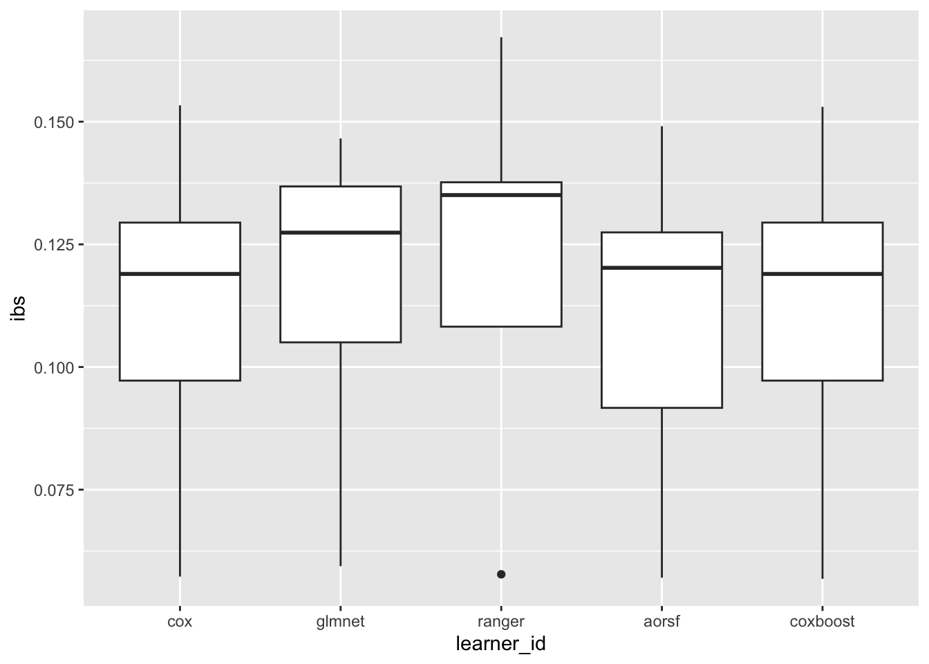
For the statistical analysis, we can use a simple rank-based analysis following Demšar (2006) with a global Friedman test to see if there are significant differences between the learners:
bma$friedman_test()
    Friedman rank sum test

data:  ibs and learner_id and task_id
Friedman chi-squared = 11.68, df = 4, p-value = 0.0199
The corresponding post-hoc test for all pairwise comparison can be performed as follows:
bma$friedman_posthoc()
Pairwise comparisons using Nemenyi-Wilcoxon-Wilcox all-pairs test for a two-way balanced complete block designdata: ibs and learner_id and task_id cox glmnet ranger aorsf
glmnet 0.855 - - -
ranger 0.180 0.751 - -
aorsf 0.931 0.373 0.023 -
coxboost 0.995 0.628 0.070 0.995
P value adjustment method: single-stepA visual approach is the critical difference plot (Demšar 2006), which shows a connecting line between the learners that are not statistically different from each other (as far as their average ranks are concerned).
autoplot(bma, type = "cd", meas = "ibs", ratio = .7)Warning in geom_segment(aes(x = 0, xend = max(rank) + 1, y = 0, yend = 0)): All aesthetics have length 1, but the data has 5 rows.
ℹ Please consider using `annotate()` or provide this layer with data containing
a single row.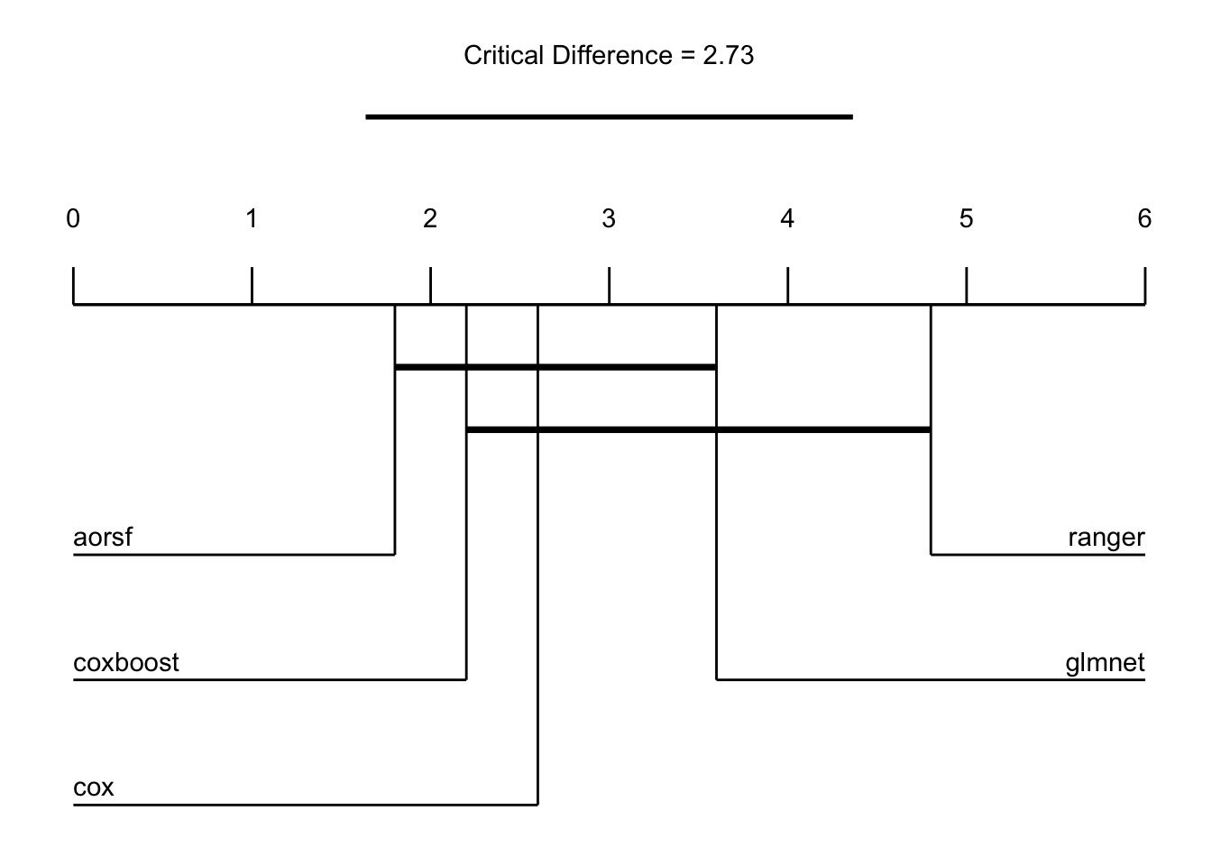
We have conducted a tiny benchmark experiment on a few survival tasks using a few learners — a good starting point for further exploration! Advanced topics we did not cover in more detail include tuning and more advanced pipelines, but we hope you got a good overview of the capabilities of mlr3proba and mlr3 in general.
sessioninfo::session_info()─ Session info ───────────────────────────────────────────────────────────────
setting value
version R version 4.4.1 (2024-06-14)
os macOS Sonoma 14.5
system aarch64, darwin20
ui X11
language (EN)
collate en_US.UTF-8
ctype en_US.UTF-8
tz Europe/Vienna
date 2024-07-08
pandoc 3.2.1 @ /opt/homebrew/bin/ (via rmarkdown)
─ Packages ───────────────────────────────────────────────────────────────────
package * version date (UTC) lib source
abind 1.4-5 2016-07-21 [1] CRAN (R 4.4.0)
aorsf 0.1.5 2024-05-30 [1] CRAN (R 4.4.0)
backports 1.5.0 2024-05-23 [1] CRAN (R 4.4.0)
bbotk 1.0.0 2024-06-28 [1] CRAN (R 4.4.0)
broom 1.0.6 2024-05-17 [1] CRAN (R 4.4.0)
BWStest 0.2.3 2023-10-10 [1] CRAN (R 4.4.0)
cachem 1.1.0 2024-05-16 [1] CRAN (R 4.4.0)
car 3.1-2 2023-03-30 [1] CRAN (R 4.4.0)
carData 3.0-5 2022-01-06 [1] CRAN (R 4.4.0)
checkmate 2.3.1 2023-12-04 [1] CRAN (R 4.4.0)
class 7.3-22 2023-05-03 [2] CRAN (R 4.4.1)
cli 3.6.3 2024-06-21 [1] CRAN (R 4.4.0)
clue 0.3-65 2023-09-23 [1] CRAN (R 4.4.0)
cluster 2.1.6 2023-12-01 [2] CRAN (R 4.4.1)
codetools 0.2-20 2024-03-31 [2] CRAN (R 4.4.1)
collapse 2.0.14 2024-05-24 [1] CRAN (R 4.4.0)
colorspace 2.1-0 2023-01-23 [1] CRAN (R 4.4.0)
cowplot 1.1.3 2024-01-22 [1] CRAN (R 4.4.0)
CoxBoost 1.5 2024-05-17 [1] Github (binderh/CoxBoost@1dc47d7)
crayon 1.5.3 2024-06-20 [1] CRAN (R 4.4.0)
data.table 1.15.4 2024-03-30 [1] CRAN (R 4.4.0)
DEoptimR 1.1-3 2023-10-07 [1] CRAN (R 4.4.0)
dictionar6 0.1.3 2021-09-13 [1] CRAN (R 4.4.0)
digest 0.6.36 2024-06-23 [1] CRAN (R 4.4.0)
diptest 0.77-1 2024-04-10 [1] CRAN (R 4.4.0)
distr6 1.8.4 2024-05-07 [1] Github (xoopR/distr6@95d7359)
dplyr 1.1.4 2023-11-17 [1] CRAN (R 4.4.0)
evaluate 0.24.0 2024-06-10 [1] CRAN (R 4.4.0)
fansi 1.0.6 2023-12-08 [1] CRAN (R 4.4.0)
farver 2.1.2 2024-05-13 [1] CRAN (R 4.4.0)
fastmap 1.2.0 2024-05-15 [1] CRAN (R 4.4.0)
flexmix 2.3-19 2023-03-16 [1] CRAN (R 4.4.0)
foreach 1.5.2 2022-02-02 [1] CRAN (R 4.4.0)
fpc 2.2-12 2024-04-30 [1] CRAN (R 4.4.0)
future 1.33.2 2024-03-26 [1] CRAN (R 4.4.0)
future.apply 1.11.2 2024-03-28 [1] CRAN (R 4.4.0)
generics 0.1.3 2022-07-05 [1] CRAN (R 4.4.0)
GGally 2.2.1 2024-02-14 [1] CRAN (R 4.4.0)
ggplot2 * 3.5.1 2024-04-23 [1] CRAN (R 4.4.0)
ggpubr 0.6.0 2023-02-10 [1] CRAN (R 4.4.0)
ggsignif 0.6.4 2022-10-13 [1] CRAN (R 4.4.0)
ggstats 0.6.0 2024-04-05 [1] CRAN (R 4.4.0)
glmnet 4.1-8 2023-08-22 [1] CRAN (R 4.4.0)
globals 0.16.3 2024-03-08 [1] CRAN (R 4.4.0)
glue 1.7.0 2024-01-09 [1] CRAN (R 4.4.0)
gmp 0.7-4 2024-01-15 [1] CRAN (R 4.4.0)
gridExtra 2.3 2017-09-09 [1] CRAN (R 4.4.0)
gtable 0.3.5 2024-04-22 [1] CRAN (R 4.4.0)
htmltools 0.5.8.1 2024-04-04 [1] CRAN (R 4.4.0)
htmlwidgets 1.6.4 2023-12-06 [1] CRAN (R 4.4.0)
iterators 1.0.14 2022-02-05 [1] CRAN (R 4.4.0)
jsonlite 1.8.8 2023-12-04 [1] CRAN (R 4.4.0)
kernlab 0.9-32 2023-01-31 [1] CRAN (R 4.4.0)
km.ci 0.5-6 2022-04-06 [1] CRAN (R 4.4.0)
KMsurv 0.1-5 2012-12-03 [1] CRAN (R 4.4.0)
knitr 1.47 2024-05-29 [1] CRAN (R 4.4.0)
kSamples 1.2-10 2023-10-07 [1] CRAN (R 4.4.0)
labeling 0.4.3 2023-08-29 [1] CRAN (R 4.4.0)
lattice 0.22-6 2024-03-20 [2] CRAN (R 4.4.1)
lava 1.8.0 2024-03-05 [1] CRAN (R 4.4.0)
lgr 0.4.4 2022-09-05 [1] CRAN (R 4.4.0)
lifecycle 1.0.4 2023-11-07 [1] CRAN (R 4.4.0)
listenv 0.9.1 2024-01-29 [1] CRAN (R 4.4.0)
magrittr 2.0.3 2022-03-30 [1] CRAN (R 4.4.0)
MASS 7.3-61 2024-06-13 [1] CRAN (R 4.4.0)
Matrix * 1.7-0 2024-04-26 [2] CRAN (R 4.4.1)
mclust 6.1.1 2024-04-29 [1] CRAN (R 4.4.0)
memoise 2.0.1 2021-11-26 [1] CRAN (R 4.4.0)
mlr3 * 0.20.0 2024-06-28 [1] CRAN (R 4.4.0)
mlr3benchmark * 0.1.6 2023-05-30 [1] CRAN (R 4.4.0)
mlr3cluster 0.1.9 2024-03-18 [1] CRAN (R 4.4.0)
mlr3data 0.7.0 2023-06-29 [1] CRAN (R 4.4.0)
mlr3extralearners 0.8.0-9000 2024-07-02 [1] Github (mlr-org/mlr3extralearners@79220c5)
mlr3filters 0.8.0 2024-04-10 [1] CRAN (R 4.4.0)
mlr3fselect 1.0.0 2024-06-29 [1] CRAN (R 4.4.0)
mlr3hyperband 0.6.0 2024-06-29 [1] CRAN (R 4.4.0)
mlr3learners 0.7.0 2024-06-28 [1] CRAN (R 4.4.0)
mlr3mbo 0.2.4 2024-07-06 [1] CRAN (R 4.4.0)
mlr3measures 0.5.0 2022-08-05 [1] CRAN (R 4.4.0)
mlr3misc 0.15.1 2024-06-24 [1] CRAN (R 4.4.0)
mlr3pipelines 0.6.0 2024-07-01 [1] CRAN (R 4.4.0)
mlr3proba * 0.6.3 2024-07-03 [1] Github (mlr-org/mlr3proba@dcd4b62)
mlr3tuning 1.0.0 2024-06-29 [1] CRAN (R 4.4.0)
mlr3tuningspaces 0.5.1.9000 2024-07-03 [1] local
mlr3verse * 0.3.0 2024-06-30 [1] CRAN (R 4.4.0)
mlr3viz 0.9.0.9000 2024-07-03 [1] Github (mlr-org/mlr3viz@aa8a86a)
modeltools 0.2-23 2020-03-05 [1] CRAN (R 4.4.0)
multcompView 0.1-10 2024-03-08 [1] CRAN (R 4.4.0)
munsell 0.5.1 2024-04-01 [1] CRAN (R 4.4.0)
mvtnorm 1.2-5 2024-05-21 [1] CRAN (R 4.4.0)
nnet 7.3-19 2023-05-03 [2] CRAN (R 4.4.1)
ooplah 0.2.0 2022-01-21 [1] CRAN (R 4.4.0)
palmerpenguins 0.1.1 2022-08-15 [1] CRAN (R 4.4.0)
paradox 1.0.0 2024-06-11 [1] CRAN (R 4.4.0)
parallelly 1.37.1 2024-02-29 [1] CRAN (R 4.4.0)
param6 0.2.4 2024-04-26 [1] Github (xoopR/param6@0fa3577)
pillar 1.9.0 2023-03-22 [1] CRAN (R 4.4.0)
pkgconfig 2.0.3 2019-09-22 [1] CRAN (R 4.4.0)
plyr 1.8.9 2023-10-02 [1] CRAN (R 4.4.0)
PMCMRplus 1.9.10 2023-12-10 [1] CRAN (R 4.4.0)
prabclus 2.3-3 2023-10-24 [1] CRAN (R 4.4.0)
pracma 2.4.4 2023-11-10 [1] CRAN (R 4.4.0)
prodlim * 2024.06.25 2024-06-24 [1] CRAN (R 4.4.0)
purrr 1.0.2 2023-08-10 [1] CRAN (R 4.4.0)
R.cache 0.16.0 2022-07-21 [1] CRAN (R 4.4.0)
R.methodsS3 1.8.2 2022-06-13 [1] CRAN (R 4.4.0)
R.oo 1.26.0 2024-01-24 [1] CRAN (R 4.4.0)
R.utils 2.12.3 2023-11-18 [1] CRAN (R 4.4.0)
R6 2.5.1 2021-08-19 [1] CRAN (R 4.4.0)
ranger 0.16.0 2023-11-12 [1] CRAN (R 4.4.0)
RColorBrewer 1.1-3 2022-04-03 [1] CRAN (R 4.4.0)
Rcpp 1.0.12 2024-01-09 [1] CRAN (R 4.4.0)
RhpcBLASctl 0.23-42 2023-02-11 [1] CRAN (R 4.4.0)
rlang 1.1.4 2024-06-04 [1] CRAN (R 4.4.0)
rmarkdown 2.27 2024-05-17 [1] CRAN (R 4.4.0)
Rmpfr 0.9-5 2024-01-21 [1] CRAN (R 4.4.0)
robustbase 0.99-3 2024-07-01 [1] CRAN (R 4.4.0)
rstatix 0.7.2 2023-02-01 [1] CRAN (R 4.4.0)
scales 1.3.0 2023-11-28 [1] CRAN (R 4.4.0)
sessioninfo 1.2.2 2021-12-06 [1] CRAN (R 4.4.0)
set6 0.2.6 2024-04-26 [1] Github (xoopR/set6@a901255)
shape 1.4.6.1 2024-02-23 [1] CRAN (R 4.4.0)
spacefillr 0.3.3 2024-05-22 [1] CRAN (R 4.4.0)
stringi 1.8.4 2024-05-06 [1] CRAN (R 4.4.0)
stringr 1.5.1 2023-11-14 [1] CRAN (R 4.4.0)
styler 1.10.3 2024-04-07 [1] CRAN (R 4.4.0)
styler.mlr 0.1.0 2024-05-16 [1] Github (mlr-org/styler.mlr@8a86087)
SuppDists 1.1-9.7 2022-01-03 [1] CRAN (R 4.4.0)
survival * 3.7-0 2024-06-05 [1] CRAN (R 4.4.0)
survivalmodels 0.1.191 2024-03-19 [1] CRAN (R 4.4.0)
survminer 0.4.9 2021-03-09 [1] CRAN (R 4.4.0)
survMisc 0.5.6 2022-04-07 [1] CRAN (R 4.4.0)
tibble 3.2.1 2023-03-20 [1] CRAN (R 4.4.0)
tidyr 1.3.1 2024-01-24 [1] CRAN (R 4.4.0)
tidyselect 1.2.1 2024-03-11 [1] CRAN (R 4.4.0)
utf8 1.2.4 2023-10-22 [1] CRAN (R 4.4.0)
uuid 1.2-0 2024-01-14 [1] CRAN (R 4.4.0)
vctrs 0.6.5 2023-12-01 [1] CRAN (R 4.4.0)
withr 3.0.0 2024-01-16 [1] CRAN (R 4.4.0)
xfun 0.45 2024-06-16 [1] CRAN (R 4.4.0)
xtable 1.8-4 2019-04-21 [1] CRAN (R 4.4.0)
yaml 2.3.9 2024-07-05 [1] CRAN (R 4.4.0)
zoo 1.8-12 2023-04-13 [1] CRAN (R 4.4.0)
[1] /Users/Lukas/Library/R/arm64/4.4/library
[2] /Library/Frameworks/R.framework/Versions/4.4-arm64/Resources/library
──────────────────────────────────────────────────────────────────────────────