Code
library(dplyr)
library(tibble)
library(ggplot2)
library(patchwork)
library(akima)
library(purrr)
library(tidyr)
library(DT)Load libraries:
library(dplyr)
library(tibble)
library(ggplot2)
library(patchwork)
library(akima)
library(purrr)
library(tidyr)
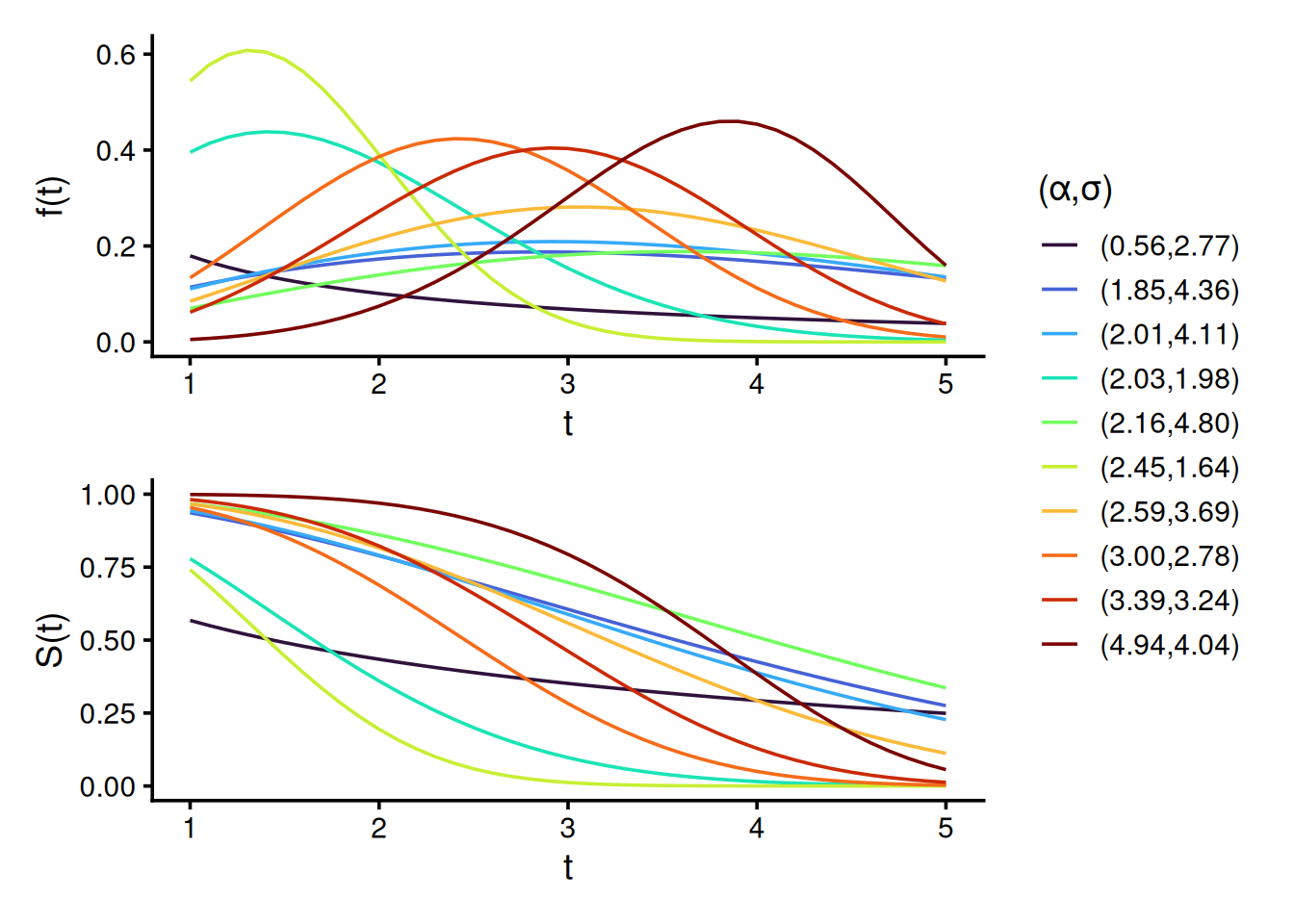
library(DT)To illustrate the diversity of the Weibull distributions used in our simulation design, we plot both the density f(t) and survival S(t) functions for 10 randomly sampled shape \alpha and scale \sigma parameter pairs. These distributions represent either the true survival, predicted survival, or censoring times across simulations. The wide parameter range induces substantial variability, ensuring a rich family of distributions and increasing the sensitivity of our evaluation to detect violations of properness. By construction, all data-generating mechanisms assume Y independent of C, satisfying the random censoring assumption.
set.seed(0L)

shape = runif(9, 0.5, 5)
scale = runif(9, 0.5, 5)

time_grid = seq(0, 6, 0.1)

params = tibble(
  id = seq_along(shape),
  shape = shape,
  scale = scale,
  group = sprintf("(%0.2f, %0.2f)", shape, scale)
)

grid = tidyr::expand_grid(params, t = time_grid)

dw = grid |>
  mutate(value = dweibull(t, shape, scale), type = "Density f(t)")

pw = grid |>
  mutate(value = pweibull(t, shape, scale, lower.tail = FALSE), type = "Survival S(t)")

plot_df = bind_rows(dw, pw) |>
  mutate(type = factor(type, levels = c("Density f(t)", "Survival S(t)")))

ggplot(plot_df, aes(x = t, y = value, color = group, group = group)) +
  geom_line(linewidth = 0.8, alpha = 0.9) +
  facet_wrap(~ type, ncol = 1, scales = "free_y") +
  scale_color_brewer(palette = "Set1") +
  scale_x_continuous(breaks = 0:6) +
  labs(
    x = expression("Time"),
    y = NULL,
    color = expression("(" * alpha * "," * sigma * ")"),
    title = "Weibull Density and Survival Curves"
  ) +
  theme_bw(base_size = 16) +
  theme(
    legend.position = "right",
    strip.text = element_text(face = "bold")
  )
#ggsave("weibull_plots.png", device = png, dpi = 600, width = 8, height = 5)This section supports the “Simulation Experiments” section of the paper.
Use properness_test.R to run the experiments. To run for different sample sizes n, use run_tests.sh. Merged simulation results for all n are available here.
Results from 10 randomly sampled simulations:
res = readRDS("results/res_sims10000_distrs1000_0.rds")

res[sample(1:nrow(res), 10), ] |>
  DT::datatable(rownames = FALSE, options = list(searching = FALSE)) |>
  formatRound(columns = 3:40, digits = c(rep(3,8), rep(5,30)))
Each row corresponds to one simulation, and the quantites are averaged across m = 1000 draws from Weibull survival distributions at a fixed sample size n \in {10, \dots, 10\,000}.
The output columns are:
sim: simulation index (k in the paper)n: sample sizen_events: number of uncensored events observed in the simulated datasetmax_t: maximum observed follow-up timem_true, m_pred: true and predicted mean survival times from the generating Weibull modelsm_true_est, m_pred_est: estimated mean survival times using the trapezoidal rule on the observed time point supportS_Y_q10, S_Y_med, S_Y_q90: values of the true event-time survival function S_Y(t) evaluated at the 10th percentile, median, and 90th percentile of the observed time points.S_C_q10, S_C_med, S_C_q90: Values of the censoring survival function S_C(t) evaluated at the 10th percentile, median, and 90th percentile of the observed time points.S_Y_tail, S_C_tail: tail survival probability at max_t for event and censoring distributionsepsilon: \hat\varepsilon = \frac{\sum_{d=1}^{1000} \left[S_Y^d(t_{\\max}^d) \times S_C^d(t_{\max}^d)\right]}{1000}{surv|pred|cens|}_{scale|shape} the scale and shape of the Weibull distributions for true, predicted and censoring times respectivelyprop_cens: proportion of censoring in each simulationtv_dist: the total variation distance between the true and the predicted Weibull distribution (closer to 0 means more similar distributions){score}_diff, {score}_sd: the mean and standard deviation of the score difference D between true and predicted distributions across drawsScoring rules analyzed:
We compute 95% confidence intervals (CIs) for the mean score difference D (true - predicted) using a t-distribution. A violation is marked statistically significant if:
res = res |>
  select(!matches("shape|scale|prop_cens|tv_dist|n_events|max_t|m_true|m_pred"))

measures = c("SBS_q10", "SBS_median", "SBS_q90", "ISBS", "RCLL", "wRCLL")
n_distrs = 1000 # `m` value from paper's experiment
tcrit = qt(0.975, df = n_distrs - 1) # 95% t-test
threshold = 1e-4

data = measures |>
  lapply(function(m) {
    mean_diff_col = paste0(m, "_diff")
    mean_sd_col = paste0(m, "_sd")

    res |>
      select(sim, n, !!mean_diff_col, !!mean_sd_col, starts_with("shift_"),
             epsilon, starts_with("S_")) |>
      select(-ends_with("tail")) |>
      mutate(
        se = .data[[mean_sd_col]] / sqrt(n_distrs),
        CI_lower = .data[[mean_diff_col]] - tcrit * se,
        CI_upper = .data[[mean_diff_col]] + tcrit * se,
        signif_violation = .data[[mean_diff_col]] > threshold & CI_lower > 0,
        # Keep relevant SBS columns
        shift_q10 = if (m == "SBS_q10") shift_q10 else NA_real_,
        S_Y_q10   = if (m == "SBS_q10") S_Y_q10 else NA_real_,
        S_C_q10   = if (m == "SBS_q10") S_C_q10 else NA_real_,
        shift_med = if (m == "SBS_median") shift_med else NA_real_,
        S_Y_med   = if (m == "SBS_median") S_Y_med else NA_real_,
        S_C_med   = if (m == "SBS_median") S_C_med else NA_real_,
        shift_q90 = if (m == "SBS_q90") shift_q90 else NA_real_,
        S_Y_q90   = if (m == "SBS_q90") S_Y_q90 else NA_real_,
        S_C_q90   = if (m == "SBS_q90") S_C_q90 else NA_real_
      ) |>
      select(!se) |>
      mutate(metric = !!m) |>
      relocate(metric, .after = 1) |>
      rename(diff = !!mean_diff_col,
             sd   = !!mean_sd_col)
  }) |>
  bind_rows()

data$metric = factor(
  data$metric,
  levels = measures,
  labels = c("SBS (Q10)", "SBS (Median)", "SBS (Q90)", "ISBS", "RCLL", "RCLL*")
)
For example, the results for the first simulation and n = 250 across all scoring rules show no violations of properness:
data |>
  filter(sim == 1, n == 250) |>
  select(-starts_with("shift"), -epsilon, -starts_with("S_")) |>
  DT::datatable(rownames = FALSE, options = list(searching = FALSE)) |>
  formatRound(columns = 4:7, digits = 5)
We summarize violations across simulations (sim), by computing for each score & sample size:
all_stats =
  data |>
  group_by(n, metric) |>
  summarize(
    n_violations = sum(signif_violation),
    violation_rate = mean(signif_violation),
    diff_mean = if (any(signif_violation)) mean(diff[signif_violation]) else NA_real_,
    diff_median = if (any(signif_violation)) median(diff[signif_violation]) else NA_real_,
    diff_min = if (any(signif_violation)) min(diff[signif_violation]) else NA_real_,
    diff_max = if (any(signif_violation)) max(diff[signif_violation]) else NA_real_,
    .groups = "drop"
  )

all_stats |>
  arrange(metric) |>
  DT::datatable(
    rownames = FALSE,
    options = list(searching = FALSE),
    caption = htmltools::tags$caption(
      style = "caption-side: top; text-align: center; font-size:150%",
      "Table 1: Empirical violations of properness")
  ) |>
formatRound(columns = 4:8, digits = 5)The theoretical shift (i.e. bias) of the global minimum x^* of the expected SBS from the true survival probability at \tau^* is (for \varepsilon \ge 0):
x^\star - S_Y(\tau^*) = - \frac{\varepsilon (1-S_Y(\tau^*))}{S_C(\tau^*) - \varepsilon} \approx - \varepsilon \cdot \frac{1 - S_Y(\tau^*)}{S_C(\tau^*)}
Filter SBS simulation data for plotting:
plot_data = data |>
  filter(grepl("^SBS", metric)) |>
  pivot_longer(
    cols = starts_with("shift_"),
    names_to = "shift_type",
    values_to = "shift",
    values_drop_na = TRUE  # only keep the relevant shift per metric
  ) |>
  mutate(
    S_Y = case_when(
      metric == "SBS (Q10)" ~ S_Y_q10,
      metric == "SBS (Median)" ~ S_Y_med,
      metric == "SBS (Q90)" ~ S_Y_q90
    ),
    S_C = case_when(
      metric == "SBS (Q10)" ~ S_C_q10,
      metric == "SBS (Median)" ~ S_C_med,
      metric == "SBS (Q90)" ~ S_C_q90
    )
  ) |>
  select(-S_Y_q10, -S_Y_med, -S_Y_q90, -S_C_q10, -S_C_med, -S_C_q90) |>
  mutate(
    metric = recode(
      metric,
      "SBS (Q10)"   = "SBS (Early, q10)",
      "SBS (Median)"= "SBS (Median, q50)",
      "SBS (Q90)"   = "SBS (Late, q90)"
    )
)ann_df = data.frame(
metric = unique(plot_data$metric)[1],
x = 0.01,
y = -0.07,
xend = 0.01,
yend = -0.175,
label = "larger bias\n(improperness)"
)
# shift vs epsilon
set.seed(42)
plot_data |>
slice_sample(prop = 0.2) |> # 20% of: 3 SBS metrics x 10 sample sizes (n) x 10000 simulations per n
ggplot(aes(x = epsilon, y = shift, color = factor(n))) +
geom_point(alpha = 0.5, size = 0.1) +
facet_wrap(~metric, scales = "fixed") +
scale_color_discrete(
name = "Sample size (n)",
) +
scale_x_continuous(
limits = c(0, 0.11),
breaks = c(0, 0.025, 0.05, 0.075, 0.1)
) +
labs(
x = "Tail product estimate ε̂ ", #expression(hat(epsilon) * " "),
y = expression(x^"*" ~ "-" ~ S[Y](tau^ ~ symbol("\052"))), # shift from optimal prediction
color = "Sample size (n)"
) +
theme_bw(base_size = 14, base_family = "Arial") +
#theme(axis.text.x = element_text(angle = 35, hjust = 1)) +
guides(color = guide_legend(override.aes = list(size = 4))) +
geom_hline(yintercept = 0, linetype = "dashed", linewidth = 0.3, color = "black") +
geom_segment(
data = ann_df,
aes(x = x, y = y, xend = xend, yend = yend),
inherit.aes = FALSE,linewidth = 1,
arrow = arrow(length = unit(0.25, "cm"))
) +
geom_text(
data = ann_df,
aes(x = x + 0.02, y = y - 0.05, label = label),
inherit.aes = FALSE,
angle = 90,
size = 6,
fontface = "bold"
)
#ggsave(filename = "epsilon_vs_bias.png", dpi = 600, height = 5, width = 10, units = "in")set.seed(42)
plot_data |>
slice_sample(prop = 0.2) |> # 3 SBS metrics x 10 sample sizes (n) x 10000 simulations per n
ggplot(aes(x = S_Y, y = shift, color = factor(n))) +
geom_point(alpha = 0.5, size = 0.3) +
facet_wrap(~metric, scales = "fixed") +
scale_color_discrete(name = "Sample size (n)") +
scale_x_continuous(
limits = c(0, 1),
breaks = c(0, 0.25, 0.5, 0.75, 1)
) +
labs(
x = expression(S[Y](tau^ ~ symbol("\052"))),
y = expression(x^"*" ~ "-" ~ S[Y](tau^ ~ symbol("\052"))),
) +
theme_bw(base_size = 14) +
theme(panel.spacing = unit(1, "lines")) +
guides(color = guide_legend(override.aes = list(size = 4))) +
geom_hline(yintercept = 0, linetype = "dashed", linewidth = 0.3, color = "black") +
geom_segment(
data = ann_df,
aes(x = x, y = y, xend = xend, yend = yend),
inherit.aes = FALSE,linewidth = 1,
arrow = arrow(length = unit(0.25, "cm"))
) +
geom_text(
data = ann_df,
aes(x = x + 0.17, y = y - 0.05, label = label),
inherit.aes = FALSE,
angle = 90,
size = 6,
fontface = "bold"
)
set.seed(42)
plot_data |>
  slice_sample(prop = 0.2) |> # 3 SBS metrics x 10 sample sizes (n) x 10000 simulations per n
  ggplot(aes(x = S_C, y = shift, color = factor(n))) +
  geom_point(alpha = 0.5, size = 0.3) +
  facet_wrap(~metric, scales = "fixed") +
  scale_color_discrete(name = "Sample size (n)") +
  scale_x_continuous(
    limits = c(0, 1),
    breaks = c(0, 0.25, 0.5, 0.75, 1)
  ) +
  labs(
    x = expression(S[C](tau^ ~ symbol("\052"))),
    y = expression(x^"*" ~ "-" ~ S[Y](tau^ ~ symbol("\052"))),
  ) +
  theme_bw(base_size = 14) +
  theme(panel.spacing = unit(1, "lines")) +
  guides(color = guide_legend(override.aes = list(size = 4))) +
  geom_hline(yintercept = 0, linetype = "dashed", linewidth = 0.3, color = "black") +
  geom_segment(
    data = ann_df,
    aes(x = x, y = y, xend = xend, yend = yend),
    inherit.aes = FALSE,linewidth = 1,
    arrow = arrow(length = unit(0.25, "cm"))
  ) +
  geom_text(
    data = ann_df,
    aes(x = x + 0.17, y = y - 0.05, label = label),
    inherit.aes = FALSE,
    angle = 90,
    size = 6,
    fontface = "bold"
  )
base_data = plot_data |>
  dplyr::filter(n == 50)

interp_shift = function(df, nx = 150, ny = 150) {
  if (nrow(df) == 0) return(NULL)

  interp_res = with(df,
    akima::interp(x = S_C, y = S_Y, z = shift, nx = nx, ny = ny, duplicate = "mean")
  )

  expand.grid(S_C = interp_res$x, S_Y = interp_res$y) |>
    mutate(shift = as.vector(interp_res$z),
           metric = unique(df$metric))
}

interp_list = base_data |>
  dplyr::group_split(metric, .keep = TRUE) |>
  purrr::map(.f = interp_shift)

surface_data = bind_rows(interp_list) |>
  dplyr::filter(!is.na(shift))

range_shift = range(surface_data$shift, na.rm = TRUE)

min_shift = range_shift[1] # most negative
max_shift = range_shift[2] # closest to zero

ggplot(surface_data, aes(x = S_C, y = S_Y, fill = shift)) +
  geom_tile() +
  facet_wrap(~ metric) +
  scale_fill_gradientn(
    colours = c("#B2182B", "grey80", "#2166AC"),
    values = scales::rescale(c(min_shift, (min_shift + max_shift)/2, max_shift)),
    limits = c(min_shift, 0), # Extend upper limit to 0
    name = expression(x^"*" ~ "-" ~ S[Y](tau^ ~ symbol("\052")))
  ) +
  labs(
    x = expression(S[C](tau^ ~ symbol("\052"))),
    y = expression(S[Y](tau^ ~ symbol("\052")))
  ) +
  theme_bw(base_size = 14) +
  theme(panel.spacing = unit(1, "lines"))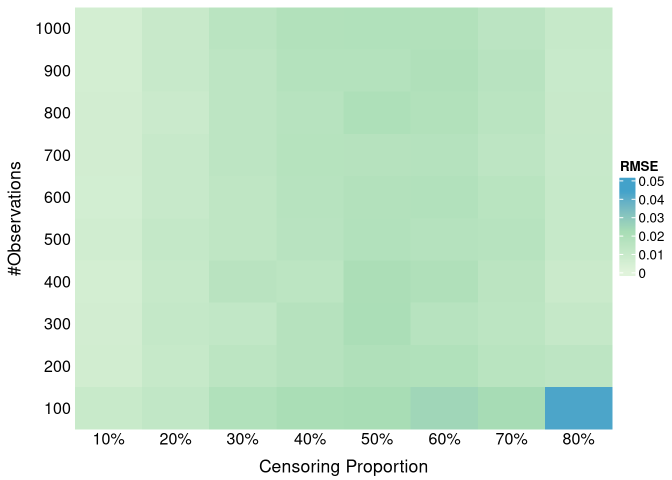
#ggsave(filename = "bias_surface_n50.png", dpi = 600, height = 5, width = 10, units = "in")base_data2 = plot_data |>
dplyr::filter(n == 100)
interp_list2 = base_data2 |>
dplyr::group_split(metric, .keep = TRUE) |>
purrr::map(.f = interp_shift)
surface_data2 = bind_rows(interp_list2) |>
dplyr::filter(!is.na(shift))
range_shift2 = range(surface_data2$shift, na.rm = TRUE)
min_shift = range_shift2[1] # most negative
max_shift = range_shift2[2] # closest to zero
ggplot(surface_data2, aes(x = S_C, y = S_Y, fill = shift)) +
geom_tile() +
facet_wrap(~ metric) +
scale_fill_gradientn(
colours = c("#B2182B", "grey80", "#2166AC"),
values = scales::rescale(c(min_shift, (min_shift + max_shift)/2, max_shift)),
limits = c(min_shift, 0), # Extend upper limit to 0
name = expression(x^"*" ~ "-" ~ S[Y](tau^ ~ symbol("\052")))
) +
labs(
x = expression(S[C](tau^ ~ symbol("\052"))),
y = expression(S[Y](tau^ ~ symbol("\052")))
) +
theme_bw(base_size = 14) +
theme(panel.spacing = unit(1, "lines"))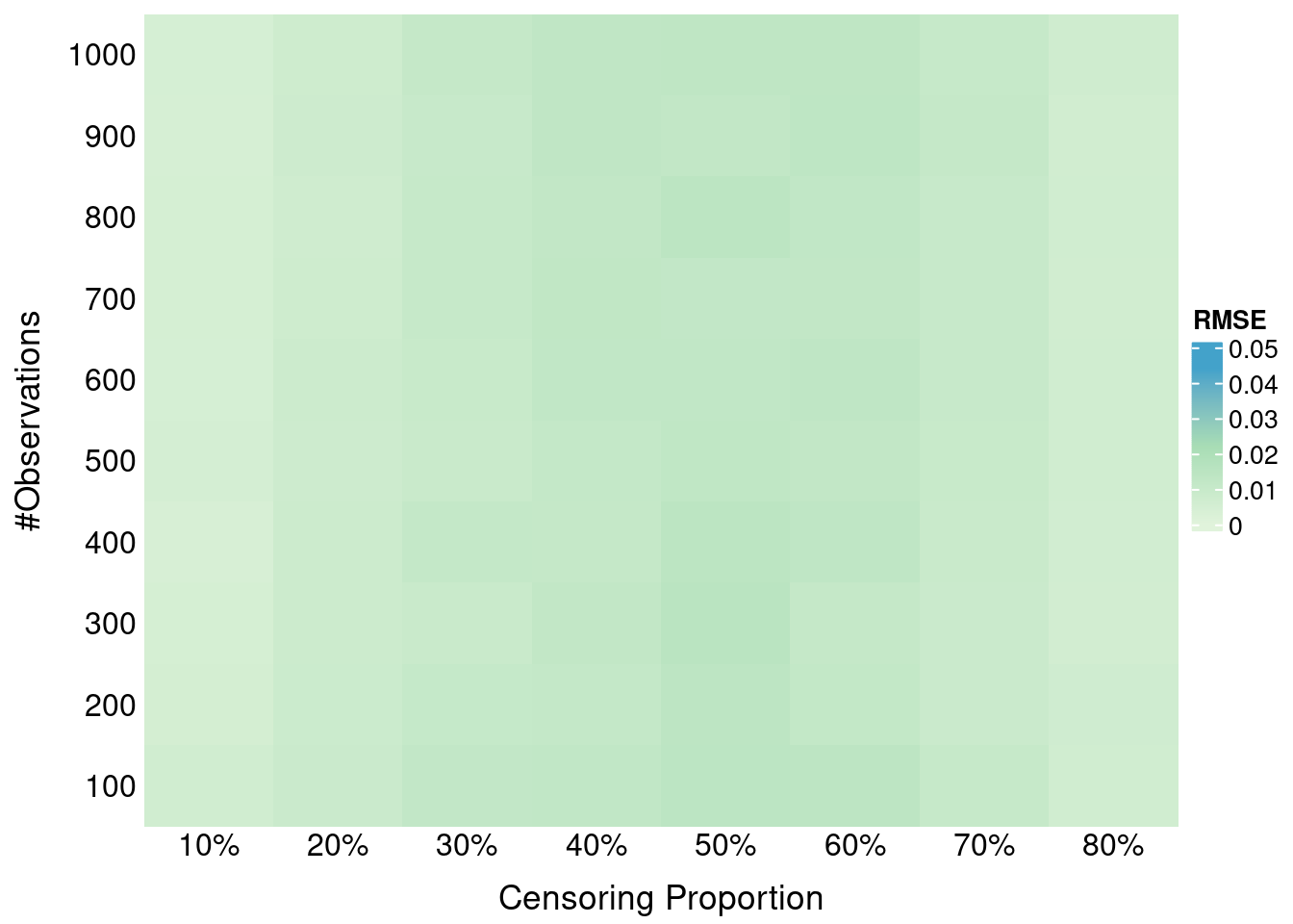
#ggsave(filename = "bias_surface_n100.png", dpi = 600, height = 5, width = 10, units = "in")plot_data |>
group_by(n) |>
summarise(
mean_hat_epsilon = mean(epsilon)
) |>
DT::datatable(
rownames = FALSE,
width = "42%",
options = list(searching = FALSE),
caption = htmltools::tags$caption(
style = "caption-side: top; text-align: center; font-size:150%",
"Empirical tail product estimate vs sample size")
) |>
formatRound(columns = 2, digits = 4)Here we investigate the impact of administritive censoring on SBS properness. Administritive censoring is applied at the 80% percentile of true times. SBS is calculated at the 10th, 50th and 90th percentile of *observed times (after application of the administrative censoring).
Use properness_test_admin_cens.R to run the experiment.
Execute: Rscript properness_test_admin_cens.R 10000 1000 10000 FALSE 42 to run for n = 10000.
Simulation results are available here.
res = readRDS("results/res_sims10000_distrs1000_n10000_0_admin_cens.rds") |>
  select(!matches("shape|scale|prop_cens|tv_dist|n_events|max_t|m_true|m_pred"))

measures = c("SBS_q10", "SBS_median", "SBS_q90", "ISBS")
n_distrs = 1000 # `m` value from paper's experiment
tcrit = qt(0.975, df = n_distrs - 1) # 95% t-test
threshold = 1e-4

data = measures |>
  lapply(function(m) {
    mean_diff_col = paste0(m, "_diff")
    mean_sd_col = paste0(m, "_sd")

    res |>
      select(sim, n, !!mean_diff_col, !!mean_sd_col, starts_with("shift_"),
             epsilon, starts_with("S_")) |>
      select(-ends_with("tail")) |>
      mutate(
        se = .data[[mean_sd_col]] / sqrt(n_distrs),
        CI_lower = .data[[mean_diff_col]] - tcrit * se,
        CI_upper = .data[[mean_diff_col]] + tcrit * se,
        signif_violation = .data[[mean_diff_col]] > threshold & CI_lower > 0,
        # Keep relevant SBS columns
        shift_q10 = if (m == "SBS_q10") shift_q10 else NA_real_,
        S_Y_q10   = if (m == "SBS_q10") S_Y_q10 else NA_real_,
        S_C_q10   = if (m == "SBS_q10") S_C_q10 else NA_real_,
        shift_med = if (m == "SBS_median") shift_med else NA_real_,
        S_Y_med   = if (m == "SBS_median") S_Y_med else NA_real_,
        S_C_med   = if (m == "SBS_median") S_C_med else NA_real_,
        shift_q90 = if (m == "SBS_q90") shift_q90 else NA_real_,
        S_Y_q90   = if (m == "SBS_q90") S_Y_q90 else NA_real_,
        S_C_q90   = if (m == "SBS_q90") S_C_q90 else NA_real_
      ) |>
      select(!se) |>
      mutate(metric = !!m) |>
      relocate(metric, .after = 1) |>
      rename(diff = !!mean_diff_col,
             sd   = !!mean_sd_col)
  }) |>
  bind_rows()

data$metric = factor(
  data$metric,
  levels = measures,
  labels = c("SBS (Early, q10)", "SBS (Median, q50)", "SBS (Late, q90)", "ISBS")
)

admin_all_stats =
  data |>
  group_by(n, metric) |>
  summarize(
    n_violations = sum(signif_violation),
    violation_rate = mean(signif_violation),
    mean_hat_epsilon = mean(epsilon),
    diff_mean = if (any(signif_violation)) mean(diff[signif_violation]) else NA_real_,
    diff_median = if (any(signif_violation)) median(diff[signif_violation]) else NA_real_,
    diff_min = if (any(signif_violation)) min(diff[signif_violation]) else NA_real_,
    diff_max = if (any(signif_violation)) max(diff[signif_violation]) else NA_real_,
    .groups = "drop"
  )

admin_all_stats |>
  arrange(metric) |>
  DT::datatable(
    rownames = FALSE,
    options = list(searching = FALSE),
    caption = htmltools::tags$caption(
      style = "caption-side: top; text-align: center; font-size:150%",
      "SBS: Empirical violations of properness for large sample size + administrative censoring")
  ) |>
formatRound(columns = 4:9, digits = 5)The only difference with the previous experiment is that S_C(t) is now being estimated using the marginal Kaplan-Meier model via survival::survfit() instead of using the true Weibull censoring distribution (see helper.R). For SBS/ISBS we use constant interpolation of the censoring survival distribution S_C(t). For RCLL* we use linear interpolation of S_C(t) to mitigate density estimation issues, i.e. for f_C(t).
Use properness_test.R to run the experiments. To run for different sample sizes n, use run_tests.sh, changing estimate_cens to TRUE. Merged simulation results for all n are available here.
Load results (same output columns as in the previous section):
res = readRDS("results/res_sims10000_distrs1000_1.rds") |>
  select(!matches("shape|scale|prop_cens|tv_dist|n_events|max_t|m_true|m_pred")) # remove columns
As before, we compute 95% confidence intervals for the score differences across m = 1000 draws per simulation:
measures = c("SBS_q10", "SBS_median", "SBS_q90", "ISBS", "RCLL", "wRCLL")
n_distrs = 1000 # `m` value from paper's experiment
tcrit = qt(0.975, df = n_distrs - 1) # 95% t-test
threshold = 1e-4

data = measures |>
  lapply(function(m) {
    mean_diff_col = paste0(m, "_diff")
    mean_sd_col = paste0(m, "_sd")

    res |>
      select(sim, n, !!mean_diff_col, !!mean_sd_col, starts_with("shift_"),
             epsilon, starts_with("S_")) |>
      select(-ends_with("tail")) |>
      mutate(
        se = .data[[mean_sd_col]] / sqrt(n_distrs),
        CI_lower = .data[[mean_diff_col]] - tcrit * se,
        CI_upper = .data[[mean_diff_col]] + tcrit * se,
        signif_violation = .data[[mean_diff_col]] > threshold & CI_lower > 0,
        # Keep relevant SBS columns, just in case
        shift_q10 = if (m == "SBS_q10") shift_q10 else NA_real_,
        S_Y_q10   = if (m == "SBS_q10") S_Y_q10 else NA_real_,
        S_C_q10   = if (m == "SBS_q10") S_C_q10 else NA_real_,
        shift_med = if (m == "SBS_median") shift_med else NA_real_,
        S_Y_med   = if (m == "SBS_median") S_Y_med else NA_real_,
        S_C_med   = if (m == "SBS_median") S_C_med else NA_real_,
        shift_q90 = if (m == "SBS_q90") shift_q90 else NA_real_,
        S_Y_q90   = if (m == "SBS_q90") S_Y_q90 else NA_real_,
        S_C_q90   = if (m == "SBS_q90") S_C_q90 else NA_real_
      ) |>
      select(!se) |>
      mutate(metric = !!m) |>
      relocate(metric, .after = 1) |>
      rename(diff = !!mean_diff_col,
             sd   = !!mean_sd_col)
  }) |>
  bind_rows()

data$metric = factor(
  data$metric,
  levels = measures,
  labels = c("SBS (Q10)", "SBS (Median)", "SBS (Q90)", "ISBS", "RCLL", "RCLL*")
)
Lastly, we summarize the significant violations across sample sizes and scoring rules:
all_stats =
  data |>
  group_by(n, metric) |>
  summarize(
    n_violations = sum(signif_violation),
    violation_rate = mean(signif_violation),
    diff_mean = if (any(signif_violation)) mean(diff[signif_violation]) else NA_real_,
    diff_median = if (any(signif_violation)) median(diff[signif_violation]) else NA_real_,
    diff_min = if (any(signif_violation)) min(diff[signif_violation]) else NA_real_,
    diff_max = if (any(signif_violation)) max(diff[signif_violation]) else NA_real_,
    .groups = "drop"
  )

all_stats |>
  arrange(metric) |>
  DT::datatable(
    rownames = FALSE,
    options = list(searching = FALSE),
    caption = htmltools::tags$caption(
      style = "caption-side: top; text-align: center; font-size:150%",
      "Table C1: Empirical violations of properness using G(t)")
  ) |>
DT::formatRound(columns = 4:8, digits = 5)Estimating S_C(t) via Kaplan-Meier produced nearly identical results to using the true distribution, with no violations for RCLL/RCLL* and only small-sample effects for SBS and ISBS.
To run the experiment use real_data_benchmark.R.
We assess the performance using three survival scoring rules (RCLL, RCLL*, ISBS), D-calibration and Harrell’s C-index on real-world survival datasets using the mlr3proba framework, tested with 10 repetitions of 5-fold cross-validation on the following learners:
Below we show the aggregated performance metrics across all tasks and learners:
res = readRDS("results/real_data_bm.rds")

res |>
  dplyr::mutate(
    learner_id = dplyr::recode(
      learner_id,
      "surv.kaplan" = "KM",
      "surv.ranger" = "RSF",
      "surv.coxph"  = "CoxPH"
    )
  )|>
  DT::datatable(rownames = FALSE, filter = "top", options = list(searching = TRUE)) |>
  DT::formatRound(columns = 3:7, digits = 3) |>
DT::formatSignif(columns = 6, digits = 3) # scientific notation for surv.dcalibOur experiment demonstrates substantial divergences in model assessment depending on the chosen metric (especially in the case of the scoring rules).
For instance, on datasets such as veteran and whas, which exhibit non-proportional hazards, RSF is more suitable to model non-linear effects compared to the CoxPH. In these cases, RCLL* identifies RSF as superior, whereas RCLL and ISBS still prefer CoxPH.
In the gbcs dataset, CoxPH achieves the best RCLL, ISBS and C-index scores, yet shows extremely poor calibration (\text{D-calib} \approx 15.7), while RCLL* ranks Kaplan-Meier as the best — possibly reflecting better-calibrated risk estimates. This discrepancy becomes even more pronounced in the lung dataset, where CoxPH again yields high RCLL/C-index/ISBS performance despite low calibration (\text{D-calib} \approx 23.5), whereas RCLL* selects RSF instead.
These findings highlight a critical need for further research: not all metrics labeled as “proper” in theory behave equally in practice.
utils::sessionInfo()R version 4.4.2 (2024-10-31)
Platform: x86_64-pc-linux-gnu
Running under: Ubuntu 24.04.3 LTS
Matrix products: default
BLAS: /usr/lib/x86_64-linux-gnu/blas/libblas.so.3.12.0
LAPACK: /usr/lib/x86_64-linux-gnu/lapack/liblapack.so.3.12.0
locale:
[1] LC_CTYPE=en_US.UTF-8 LC_NUMERIC=C
[3] LC_TIME=en_DK.UTF-8 LC_COLLATE=en_US.UTF-8
[5] LC_MONETARY=en_DK.UTF-8 LC_MESSAGES=en_US.UTF-8
[7] LC_PAPER=en_DK.UTF-8 LC_NAME=C
[9] LC_ADDRESS=C LC_TELEPHONE=C
[11] LC_MEASUREMENT=en_DK.UTF-8 LC_IDENTIFICATION=C
time zone: Europe/Oslo
tzcode source: system (glibc)
attached base packages:
[1] stats graphics grDevices utils datasets methods base
other attached packages:
[1] DT_0.33 tidyr_1.3.1 purrr_1.0.2 akima_0.6-3.6
[5] patchwork_1.3.2 ggplot2_4.0.2 tibble_3.3.0 dplyr_1.1.4
loaded via a namespace (and not attached):
[1] gtable_0.3.6 jsonlite_2.0.0 compiler_4.4.2 tidyselect_1.2.1
[5] jquerylib_0.1.4 scales_1.4.0 yaml_2.3.12 fastmap_1.2.0
[9] lattice_0.22-6 R6_2.6.1 labeling_0.4.3 generics_0.1.3
[13] knitr_1.51 htmlwidgets_1.6.4 bslib_0.10.0 pillar_1.11.0
[17] RColorBrewer_1.1-3 rlang_1.1.7 sp_2.1-4 cachem_1.1.0
[21] xfun_0.57 sass_0.4.10 S7_0.2.1 cli_3.6.5
[25] withr_3.0.2 magrittr_2.0.4 crosstalk_1.2.1 digest_0.6.39
[29] grid_4.4.2 lifecycle_1.0.5 vctrs_0.7.1 evaluate_1.0.5
[33] glue_1.8.0 farver_2.1.2 rmarkdown_2.30 tools_4.4.2
[37] pkgconfig_2.0.3 htmltools_0.5.9